FROM CELL MEMBRANES TO ULTRACOLD GASES: CLASSICAL AND QUANTUM - - PowerPoint PPT Presentation

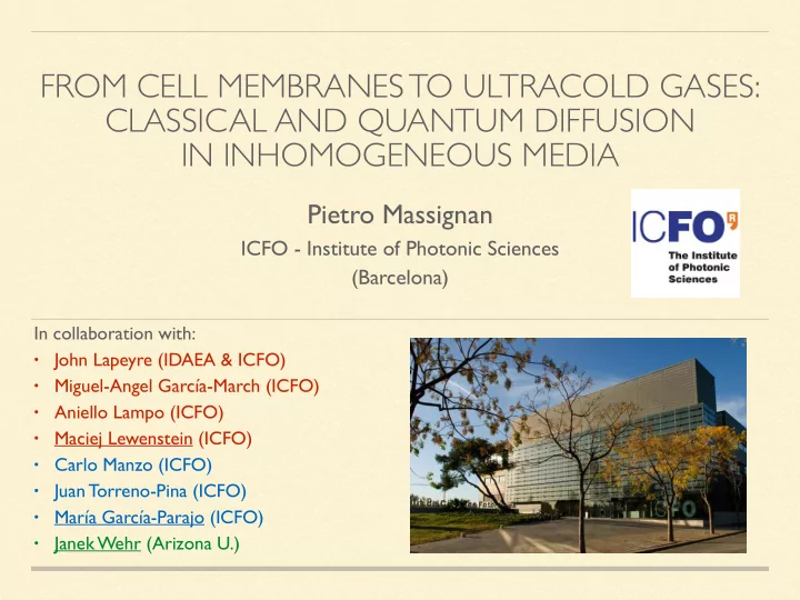
FROM CELL MEMBRANES TO ULTRACOLD GASES:
 CLASSICAL AND QUANTUM DIFFUSION
 IN INHOMOGENEOUS MEDIA

Pietro Massignan

ICFO - Institute of Photonic Sciences (Barcelona)

In collaboration with:

• John Lapeyre (IDAEA & ICFO)
• Miguel-Angel García-March (ICFO)
• Aniello Lampo (ICFO)
• Maciej Lewenstein (ICFO)
• Carlo Manzo (ICFO)
• Juan Torreno-Pina (ICFO)
• María García-Parajo (ICFO)
• Janek Wehr (Arizona U.)

Outlook

• A. Classical
• Anomalous diffusion in biological systems
• Kinetic Ising Models
• B. Quantum
• Quantum Kinetic Ising Models
• Quantum Brownian Motion

2

Ordinary Random Walk

3 E-MSD(tlag = m∆t) = 1 J

J

X

j=1

• xj (ti + m∆t) − xj (ti)

2

Time-averaged mean squared displacement along a single trajectory: Ensemble-averaged mean squared displacement over J trajectories:

An ordinary RW is

• diffusive: MSD~tβ, with β=1
• ergodic: T-MSD and E-MSD coincide at long times
• stationary: MSD independent of the total observation time (at large times)

T-MSD(tlag = m∆t) = 1 N − m

N−m

X

i=1

• x (ti + m∆t) − x (ti)

2

Diffusion in structured media

4

A random walker may be strongly affected by:

• repeated interactions
• transient binding
• clustering
• crowding
• multi-scale, or scale-free, disorder

Live cell membrane

5

A random walker may be strongly affected by:

• repeated interactions
• transient binding
• clustering
• crowding
• multi-scale, or scale-free, disorder

Trans-membrane receptors

Single particle tracking of
 pathogen-recognizing receptors


• n live cellular membranes

60 frames/s
 20nm position accuracy

6

(M. García-Parajo’s group @ ICFO)

Manzo, Torreno-Pina, PM, Lapeyre, Lewenstein & García-Parajo, Phys. Rev. X (2015)

Different scaling of T-MSD and E-MSD ➟ weak ergodicity breaking!

7

The TE-MSD depends on the total observation time T ➟ non-stationary! Time-averaged MSD Ensemble-averaged MSD Sampling of J=600 trajectories TE-MSD ∼ DTE(T) · tlag Time&Ensemble averaged MSD:

RTH

Continuous-Time Random Walk

• CTRW: a fat-tailed distribution of waiting times ~t
• 1-β with β≤1 (so that <twait>=∞)


induces non-stationary (thus non-ergodic) subdiffusion
 with E-MSD~t

β and TE-MSD~DTE(T)*tlag, with DTE~T β-1

• Widely used model for transport in disordered media (initially developed for amorphous solids)

• However, are trapping events present in the ICFO experiment?


• nly 5% of the trajectories contain events


compatible with transient trapping
 
 and excluding these trajectories yields
 a very similar E-MSD exponent β


• For CTRW, the long-time dynamics is 


dominated by anomalous trapping events,
 so that the escape-time distribution at long times
 becomes independent of the trapping radius RTH

8

Montroll & Weiss, 1965; Montroll & Scher, 1973

Strongly varying diffusivity

• Maps of receptor motion on the cell membrane highlight the 


presence of patches with strongly varying diffusivity

• Many possible reasons: crossing regions of low/high 


viscosity, transient binding, clustering, …

• Employ a likelihood-based Bayesian algorithm to detect


time-dependent changes of diffusivity within a single trajectory:

9

Theoretical model

• Ordinary Brownian motion with a diffusivity that varies randomly,


but it’s constant on time intervals with random duration
 (or patches with random sizes)

• Assume a distribution of diffusion coefficients



 and a conditional distribution of transit times


• Three possible regimes:

(0) γ<σ: the long-time dynamics is compatible with regular Brownian motion (β=1)
 
 (I) σ<γ<σ+1: the average transit-time diverges ➟ non-ergodic sub-diffusion (β=σ/γ)
 
 (II) γ>σ+1: both <τ> and <(rarea)2> diverge ➟ non-ergodic sub-diffusion (β=1-1/γ)

PD(D) ∼ Dσ−1e−D/b

Pτ(τ|D) ∼ Dγe−τDγ/k

power law at small D
 fast decay at large D
 
 mean transit time ~D-γ
 each area has radius r~(τD)-1/2

PM, Manzo, Torreno-Pina, García-Parajo, Lewenstein & Lapeyre, Phys. Rev. Lett. (2014) 10

Comparison with experiments

Manzo, Torreno-Pina, PM, Lapeyre, Lewenstein & García-Parajo, Phys. Rev. X (2015)

Simulation of
 WT dynamics
 σ=1.16
 γ=1.38 regime (I) ☟ non-ergodic
 subdiffusion with β=σ/γ=0.84

Instead, mutated receptors with impaired function (Δrep) may be best simulated
 with γ<σ, i.e., they perform usual ergodic and diffusive Brownian motion
 
 Transport properties strongly linked to molecular function

11

Include receptor/membrane interactions?

12

⬆ ⬆ ⬆ ⬇ ⬇

Model the membrane as an Ising lattice: H = −J X

i

σiσi+1 Link diffusivity to local membrane state (e.g. faster diffusion on ⬆ background) Allow walker to locally modify
 the membrane state σi =↑, ↓ [see Poster P.03 “Random walks in Random Environments” by M.-A. García-March]

Kinetic Ising Model for the membrane

• Kinetic Ising Model:
• Interacting membrane:
• Detailed balance at equilibrium:
• Recursive system of differential equations: e.g.,
• Exact time-dependent solutions may be found for: infinite lattice, single spin fixed, (time-

delayed) spin correlations, spin systems in a magnetic field, …

• R. Glauber, Time-dependent statistics of the Ising model, J. Math. Phys. (1963)

13 ˙ P(σ, t) = X

σ0

[w(σ0 → σ)P(σ0, t) − w(σ → σ0)P(σ, t)]

w: transition rate α/2: single spin-flip rate γ>0: IFM
 γ<0: AFM

w(σi → −σi) = α 2 h 1 − γ 2 σi(σi−1 + σi+1) i P(σ, t) = 1 2N X

{σ0}

(1 + σ1σ0

1) . . . (1 + σNσ0 N)P(σ0, t) = 1

2N 8 < :1 + X

i

σiqi(t) + X

i6=k

σiσkri,k(t) + . . . 9 = ;

qi(t) = hσi(t)i ri,k(t) = hσi(t)σk(t)i

α−1 ˙ qi(t) = −qi(t) + γ/2[qi−1(t) + qi+1(t)] Peq(σ1, . . . , σi, . . . , σn)w(σi → −σi) = Peq(σ1, . . . , −σi, . . . , σn)w(−σi → σi) Peq(σ1, . . . , σi, . . . , σn) ∝ exp[βJσi(σi−1 + σi+1)]

Kinetic Ising Model for membrane+walker

• Master equation:
• The walker may act as a localized potential for the spins, or it may change the tunneling

between the neighboring spins

• If either the spins or the walker dynamics is fast, we may use an adiabatic approximation
• E.g., and
• polaronic behavior (rapid formation of a dressing cloud, dragged along by the walker)
• In the opposite limit instead, the walker spreads very fast, and will act as a diffuse potential

(mean-field) for the membrane

14 ˙ P(σ, x, t) = [γsLs + γwLw]P(σ, x, t)

s: spins (=membrane) w: walker x: position of the walker

γs γw ! L = γs  Ls + γw γs Lw

• P(σ, x, t) ∼ Pw(x, t|σ)P (eq)

s

(σ|x)

(Quantum) Kinetic Ising Models

• Ansatz:
• The KIM master equation may be written as
• If the KIM satisfies a detailed-balanced condition, then H is a (real) symmetric matrix, so that

the KIM-ME may be seen as a Schrödinger equation in imaginary time, which converges exponentially to the thermal equilibrium solution. Diagonalization of H is then equivalent to the complete solution of the KIM-ME

• Classical spins may be promoted to non-commuting Pauli matrices to obtain quantum models
• Quantum states built from thermal states of classical Hamiltonians, e.g.,


fulfill the area law in any dimension, even at criticality, and can be represented efficiently as matrix product states (MPS), or projected entangled pair states (PEPS)

15 P(σ, t) = q Peq(σ)φ(σ, t) ˙ φ(σ, t) = − X

σ0

Hσσ0φ(σ0, t)

Hσσ0 = X

σ00

w(σ → σ00)δσσ0 − w(σ0 → σ) s Peq(σ0) Peq(σ)

Augusiak, Cucchietti, Haake & Lewenstein, New J. Phys. (2010)

|Ψi = 1 pZN X

σ

e−βH(σ)/2|σi

Quantum Brownian Motion

• A small system interacting with a large thermal bath:
• Simplest interaction:
• ME for the reduced density matrix:
• Born approx.:
• Markov approx.: the bath evolves on timescales much faster than the system, and as such

effectively retains no memory of the system’s dynamics

• The spectral density contains all details of the bath-system coupling:

16 H = HS + HB + HI HI = − X

k

κkxkx

xk: position of the kth oscillator κk: coupling constant x: position of the system

˙ ρS(t) = − 1 ~2 Z t ds TrB[HI(t), [HI(s), ρ(s)]] ρ(t) ' ρS(t) ⌦ ρB(0) J(ω) ≡ X

k

κ2

k

2mkωk δ(ω − ωk)

Born-Markov QME

• Weak-coupling limit (second-order perturbation in HI)
• Ohmic spectral density with Lorentz-Drude cut-off:
• Consider a particle of mass m in a harmonic trap of frequency Ω. In the high-temperature

limit one obtains the celebrated Caldeira-Leggett QME:
 


• A quantum stochastic process is said to be Markovian only if the underlying noise is white,

and if the process is described by a time-independent ME of the Lindblad form

• Note that there exists an exact solution of the QBM problem, which however has a time-

dependent Liouvillian. Strictly-speaking, QBM is not a quantum Markov process.

J(ω) = mγω π Λ2 ω2 + Λ2 kBT ~Λ ~Ω ˙ ρS = − i ~[Hsys, ρS] − iγ 2~[x, {p, ρS}] − mγkBT ~2 [x, [x, ρS]]

momentum damping normal diffusion

17

Impurities in an inhomogeneous 1D BEC

PM, Lampo, Wehr & Lewenstein, Phys. Rev. A (2015)

Catani et al., Phys. Rev. A (2012)

# How to treat a spatially-dependent profile of the bath?
 Coupling which is a non-linear function of the system’s position: 
 
 
 # How to deal with the low temperatures of a quantum gas?
 Non-Markovian effects will become important here!
 
 # And what if the spectral density is not Ohmic?
 (i.e., the noise is not white)

HI = − X

k

κkxkf(x)

Aspect ratio of the impurity, ln(δp2/δx2),
 for a quadratic coupling with the environment: δx2<δp2 δx<1

18

Open questions

• A. Classical
• Anomalous diffusion in biological systems
• Kinetic Ising Models

• B. Quantum
• Quantum Kinetic Ising Models
• Quantum Brownian Motion

19

Q: mechanisms leading to sub- or super-diffusion, Levy flights, non-stationarity and non-ergodicity? Q: mechanisms generating interactions between walkers and substrates? Q: novel exactly or efficiently solvable quantum Hamiltonians? Q: importance of non-Markovian effects at low temperatures?

Conclusions

• Walkers on largely heterogeneous substrate can exhibit

strongly subdiffusive and non-ergodic behavior, even without transient immobilization

• We are working towards describing membrane-walkers

interactions by means of Kinetic Ising Models (KIMs)

• KIMs may be generalized to the quantum domain
• Quantum Brownian Motion in presence of an inhomogeneous

background may be described by couplings which are polynomial functions of the system variables

20 PM, Manzo, Torreno-Pina, García-Parajo, Lewenstein & Lapeyre, Phys. Rev. Lett. (2014) Manzo, Torreno-Pina, PM, Lapeyre, Lewenstein & García-Parajo, Phys. Rev. X (2015) PM, Lampo, Wehr & Lewenstein, Phys. Rev. A (2015)

In collaboration with:

21

John Lapeyre (ICFO&IDAEA) Maciej Lewenstein Miguel-Angel
 García March Carlo Manzo María García-Parajo Juan Torreno-Pina Quantum Optics Theory @ ICFO Aniello Lampo Single Molecule Biophotonics @ ICFO Math @ Arizona U. Janek Wehr

THANK YOU!