23 24 25 26 27 28 29 30 31 32 33 34 35 36 37 38 39 40 41 M - - PDF document

23 24 25 26 27 28 29 30 31 32 33 34 35 36 37 38 39 40 41
SMART_READER_LITE
LIVE PREVIEW

23 24 25 26 27 28 29 30 31 32 33 34 35 36 37 38 39 40 41 M - - PDF document

M I Variational Methods and Optimization in Imaging Institut Henri Poincar e, Paris, February 48, 2019 A 1 2 3 4 5 6 Stable Models and Algorithms for 7 8 Backward Diffusion Evolutions 9 10 11 12 13 14 Joachim Weickert 15 16


slide-1
SLIDE 1

Variational Methods and Optimization in Imaging Institut Henri Poincar´ e, Paris, February 4–8, 2019

M I

A

Stable Models and Algorithms for Backward Diffusion Evolutions

Joachim Weickert Mathematical Image Analysis Group Saarland University, Saarbr¨ ucken, Germany joint work with Martin Welk (UMIT, Hall, Austria) Leif Bergerhoff (Saarland University) Marcelo C´ ardenas (Saarland University) Guy Gilboa (Technion, Haifa, Israel)

partial funding: DFG Leibniz Award and ERC Advanced Grant INCOVID

1 2 3 4 5 6 7 8 9 10 11 12 13 14 15 16 17 18 19 20 21 22 23 24 25 26 27 28 29 30 31 32 33 34 35 36 37 38 39 40 41 Introduction (1)

M I

A

Introduction

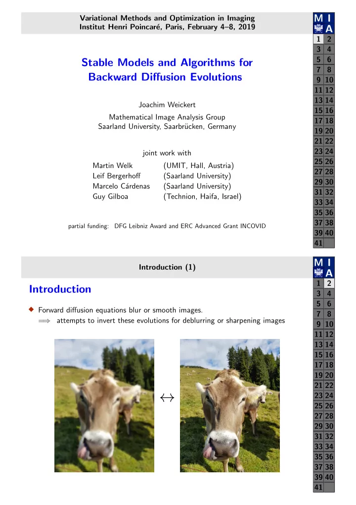
  • Forward diffusion equations blur or smooth images.

= ⇒ attempts to invert these evolutions for deblurring or sharpening images

1 2 3 4 5 6 7 8 9 10 11 12 13 14 15 16 17 18 19 20 21 22 23 24 25 26 27 28 29 30 31 32 33 34 35 36 37 38 39 40 41

slide-2
SLIDE 2

Introduction (2)

M I

A

Problems

  • Backward diffusion is typically regarded as ill-posed:
  • Solution does not exist for non-smooth initial data.
  • If it exists, it is highly sensitive w.r.t. perturbations.
  • Thus, many researchers refrain from using backward diffusion.

Goals

  • show how these problems can be
  • handled by sophisticated numerics
  • or circumvented by smart modelling
  • demonstate these principles with two prototypical applications:
  • advanced numerics for the FAB diffusion of Gilboa et al. 2002
  • novel convex model for backward diffusion (Bergerhoff et al. 2018)

1 2 3 4 5 6 7 8 9 10 11 12 13 14 15 16 17 18 19 20 21 22 23 24 25 26 27 28 29 30 31 32 33 34 35 36 37 38 39 40 41 Outline

M I

A

Outline

  • FAB Diffusion
  • Continuous Model
  • Explicit Scheme
  • Efficient Numerics
  • Experiments
  • Backward Diffusion with Convex Energy
  • Model and Theory
  • Numerical Algorithm
  • Experiment
  • Conclusions

1 2 3 4 5 6 7 8 9 10 11 12 13 14 15 16 17 18 19 20 21 22 23 24 25 26 27 28 29 30 31 32 33 34 35 36 37 38 39 40 41

slide-3
SLIDE 3

Outline

M I

A

Outline

  • FAB Diffusion
  • Continuous Model
  • Explicit Scheme
  • Efficient Numerics
  • Experiments
  • Backward Diffusion with Convex Energy
  • Model and Theory
  • Numerical Algorithm
  • Experiment
  • Conclusions

1 2 3 4 5 6 7 8 9 10 11 12 13 14 15 16 17 18 19 20 21 22 23 24 25 26 27 28 29 30 31 32 33 34 35 36 37 38 39 40 41 FAB Diffusion: Continuous Model (1)

M I

A

FAB Diffusion: Continuous Model

The Perona–Malik Filter (1990)

  • Consider open image domain Ω ⊂ R2 and some bounded image f : Ω → R.
  • Create family of filtered versions u(x, t) of f(x) as solution of

∂tu = div

  • g(|∇u|2) ∇u
  • n Ω × (0, ∞),

u(x, 0) = f(x)

  • n Ω,

n⊤∇u = 0

  • n ∂Ω × (0, ∞),

where n denotes the outer normal vector to the image boundary ∂Ω.

  • diffusivity g is monotonically decreasing positive function of |∇u|2
  • smoothes within flat regions and enhances edges between them
  • gradient descent of a possibly nonconvex but monotone energy

E(u) =

Ψ(|∇u|2) dx where the penaliser (potential) Ψ(|∇u|2) satisfies Ψ′(|∇u|2) = g(|∇u|2) . 1 2 3 4 5 6 7 8 9 10 11 12 13 14 15 16 17 18 19 20 21 22 23 24 25 26 27 28 29 30 31 32 33 34 35 36 37 38 39 40 41

slide-4
SLIDE 4

FAB Diffusion: Continuous Model (2)

M I

A

Forward-and-Backward (FAB) Diffusion (Gilboa / Sochen / Zeevi 2002)

  • goal:

stronger sharpening than classical Perona-Malik filters

  • equip Perona-Malik diffusion

∂tu = div

  • g(|∇u|2) ∇u
  • with a diffusivity that takes positive and negative values.
  • fairly mild assumptions in this talk:

g ∈ C1[0, ∞), g(0) = c1 > 0, g( . ) ≥ −c2 with c1 > c2 ≥ 0.

  • corresponds to nonconvex and nonmonotone potential Ψ(|∇u|2)

1 2 3 4 5 6 7 8 9 10 11 12 13 14 15 16 17 18 19 20 21 22 23 24 25 26 27 28 29 30 31 32 33 34 35 36 37 38 39 40 41 FAB Diffusion: Continuous Model (3)

M I

A

How Unpleasant can this Become ?

Diffusivity g(s2) Diffusivity g(s2) Diffusivity g(s2) Potential Ψ(s2) Potential Ψ(s2) Potential Ψ(s2)

1 2 3 4 5 6 7 8 9 10 11 12 13 14 15 16 17 18 19 20 21 22 23 24 25 26 27 28 29 30 31 32 33 34 35 36 37 38 39 40 41

slide-5
SLIDE 5

FAB Diffusion: Continuous Model (4)

M I

A

Theoretical Results so Far

  • cannot be covered by standard theory for diffusion filters (W. 1998)
  • no continuous well-posedness theory
  • Gilboa / Sochen / Zeevi

(IEEE TIP 2002): standard implementations violate extremum principle

  • Gilboa / Sochen / Zeevi

(JMIV 2004): experimental stabilisation with a fidelity term and biharmonic regularisation Can we establish a fully discrete theory ? Does this lead to practical algorithms for images? 1 2 3 4 5 6 7 8 9 10 11 12 13 14 15 16 17 18 19 20 21 22 23 24 25 26 27 28 29 30 31 32 33 34 35 36 37 38 39 40 41 Outline

M I

A

Outline

  • FAB Diffusion
  • Continuous Model
  • Explicit Scheme
  • Efficient Numerics
  • Experiments
  • Backward Diffusion with Convex Energy
  • Model and Theory
  • Numerical Algorithm
  • Experiment
  • Conclusions

1 2 3 4 5 6 7 8 9 10 11 12 13 14 15 16 17 18 19 20 21 22 23 24 25 26 27 28 29 30 31 32 33 34 35 36 37 38 39 40 41

slide-6
SLIDE 6

FAB Diffusion: Explicit Scheme (1)

M I

A

FAB Diffusion: Explicit Scheme

Goal

  • establish comprehensive theory for an explicit discretisation of FAB diffusion

Explicit Scheme Explicit finite difference discretisation of diffusion equation ∂tu = ∂x

  • g(|∇u|2) ∂xu
  • + ∂y
  • g(|∇u|2) ∂yu
  • in some inner pixel (i, j) at time level k yields the scheme

uk+1

i,j

− uk

i,j

τ = 1 h1

  • gk

i+1,j + gk i,j

2 uk

i+1,j − uk i,j

h1 − gk

i,j + gk i−1,j

2 uk

i,j − uk i−1,j

h1

  • +

1 h2

  • gk

i,j+1 + gk i,j

2 uk

i,j+1 − uk i,j

h2 − gk

i,j + gk i,j−1

2 uk

i,j − uk i,j−1

h2

  • with grid sizes h1, h2 and time step size τ.

1 2 3 4 5 6 7 8 9 10 11 12 13 14 15 16 17 18 19 20 21 22 23 24 25 26 27 28 29 30 31 32 33 34 35 36 37 38 39 40 41 FAB Diffusion: Explicit Scheme (2)

M I

A

Where Do Problems Arise ?

  • The standard discretisation of g(|∇u|2) is given by

gk

i,j := g

uk

i+1,j − uk i−1,j

2 h1

  • 2

+

  • uk

i,j+1 − uk i,j−1

2 h2

  • 2
  • can be positive at extrema
  • .
  • It can create negative diffusivities in extrema, which give rise to instabilities.

Is There a Remedy ?

  • A nonstandard discretisation produces a vanishing gradient in extrema:

gk

i,j :=

g

  • max
  • uk

i+1,j − uk i,j

h1 · uk

i,j − uk i−1,j

h1 , 0

  • + max
  • uk

i,j+1 − uk i,j

h2 · uk

i,j − uk i,j−1

h2 , 0

  • .
  • same quadratic consistency order as standard discretisation

1 2 3 4 5 6 7 8 9 10 11 12 13 14 15 16 17 18 19 20 21 22 23 24 25 26 27 28 29 30 31 32 33 34 35 36 37 38 39 40 41

slide-7
SLIDE 7

FAB Diffusion: Explicit Scheme (3)

M I

A

Two Technical Definitions

  • The grey values of f = (fi) ∈ RN are restricted to a finite interval of length

R := max

i

fi − min

i

fi.

  • Since g is continuous and c1 > c2 ≥ 0 , there exists a constant ω > 0 such that

g(s2) > c2 ∀ s ∈ (0, ωR).

|∇u| c1 −c2 c2 ωR

1 2 3 4 5 6 7 8 9 10 11 12 13 14 15 16 17 18 19 20 21 22 23 24 25 26 27 28 29 30 31 32 33 34 35 36 37 38 39 40 41 FAB Diffusion: Explicit Scheme (4)

M I

A

Theorem [Theory for the Explicit FAB Scheme] With the preceding assumptions and definitions, consider the explicit scheme for FAB diffusion with nonstandard discretisation. If the time step size τ satisfies τ ≤ ω2 h4

1 h4 2

2 c1 ·

  • h2

1 + h2 2

  • ·
  • ω2 h2

1 h2 2 + h2 1 + h2 2

, then this scheme has the following properties:

  • Well-Posedness

For every k ∈ N0, the solution uk+1 depends in a continuous way on perturbations

  • f the initial image f.
  • Average Grey Value Invariance

1 N

N

  • j=1

uk

j =

1 N

N

  • j=1

fj =: µ ∀ k ∈ N0. 1 2 3 4 5 6 7 8 9 10 11 12 13 14 15 16 17 18 19 20 21 22 23 24 25 26 27 28 29 30 31 32 33 34 35 36 37 38 39 40 41

slide-8
SLIDE 8

FAB Diffusion: Explicit Scheme (5)

M I

A

  • Maximum-Minimum Principle

min

j

fj ≤ uk

i ≤ max j

fj ∀ i, ∀ k ∈ N0.

  • Lyapunov Sequence

V k := max

j

uk

j − min j

uk

j

is a Lyapunov sequence: decreasing in k and bounded from below.

  • Convergence to a Constant Steady State

lim

k→∞ uk i = µ

∀ i. 1 2 3 4 5 6 7 8 9 10 11 12 13 14 15 16 17 18 19 20 21 22 23 24 25 26 27 28 29 30 31 32 33 34 35 36 37 38 39 40 41 Outline

M I

A

Outline

  • FAB Diffusion
  • Continuous Model
  • Explicit Scheme
  • Efficient Numerics
  • Experiments
  • Backward Diffusion with Convex Energy
  • Model and Theory
  • Numerical Algorithm
  • Experiment
  • Conclusions

1 2 3 4 5 6 7 8 9 10 11 12 13 14 15 16 17 18 19 20 21 22 23 24 25 26 27 28 29 30 31 32 33 34 35 36 37 38 39 40 41

slide-9
SLIDE 9

FAB Diffusion: Efficient Numerics (1)

M I

A

FAB Diffusion: Efficient Numerics

  • Our explicit FAB scheme with nonstandard discretisation has a clean theory.
  • However, it must satisfy a severe time step size restriction:

This can lead to impractically small time steps: 10−6,...,10−5

  • Reason:
  • based on worst case a priori estimates
  • restrictions are not needed everywhere and at all time steps
  • Remedy:
  • Replace pessimistic a priori estimates by realistic a posteriori estimates.
  • Act as locally/adaptive as possible in space and time.
  • Realisation:

two-pixel interactions. 1 2 3 4 5 6 7 8 9 10 11 12 13 14 15 16 17 18 19 20 21 22 23 24 25 26 27 28 29 30 31 32 33 34 35 36 37 38 39 40 41 FAB Diffusion: Efficient Numerics (2)

M I

A

Motivation for Two-Pixel Interactions

  • most local diffusion interaction that respects a conservation law.

← → ui,j ui

+ 1,j

  • r
  • ui,j

ui,j+

1

  • The explicit scheme performs four two-pixel interactions simultaneously:

uk+1

i,j

= uk

i,j + τ

  • gk

i+1,j + gk i,j

2 · uk

i+1,j − uk i,j

h2

1

− gk

i,j + gk i−1,j

2 · uk

i,j − uk i−1,j

h2

1

+ gk

i,j+1 + gk i,j

2 · uk

i,j+1 − uk i,j

h2

2

− gk

i,j + gk i,j−1

2 · uk

i,j − uk i,j−1

h2

2

  • 1

2 3 4 5 6 7 8 9 10 11 12 13 14 15 16 17 18 19 20 21 22 23 24 25 26 27 28 29 30 31 32 33 34 35 36 37 38 39 40 41

slide-10
SLIDE 10

FAB Diffusion: Efficient Numerics (3)

M I

A

Basic Idea behind Two-Pixel Scheme

  • Decouple explicit scheme into sequential (asynchroneous) two-pixel interactions.

Then stability follows trivially from the stability of each interaction.

  • In each interaction, choose the largest time step ensuring two stability criteria:
  • For a positive diffusivity, the order of grey values must not be flipped.
  • For a negative diffusivity, we have a non-extremal pixel.

It must not become larger/smaller than its largest/smallest neighbour.

  • This gives highly localised time step size restrictions in space and time.
  • To avoid directional bias, randomise the order of two-pixel interactions.
  • Introduce sync times at which each all pixels reach the same time level.

Use e.g. the stability bounds of an explicit forward diffusion scheme.

  • selection probability for two-pixel interaction:

proportional to remaining time until synchronisation. 1 2 3 4 5 6 7 8 9 10 11 12 13 14 15 16 17 18 19 20 21 22 23 24 25 26 27 28 29 30 31 32 33 34 35 36 37 38 39 40 41 Outline

M I

A

Outline

  • FAB Diffusion
  • Continuous Model
  • Explicit Scheme
  • Efficient Numerics
  • Experiments
  • Backward Diffusion with Convex Energy
  • Model and Theory
  • Numerical Algorithm
  • Experiment
  • Conclusions

1 2 3 4 5 6 7 8 9 10 11 12 13 14 15 16 17 18 19 20 21 22 23 24 25 26 27 28 29 30 31 32 33 34 35 36 37 38 39 40 41

slide-11
SLIDE 11

FAB Diffusion: Experiments (1)

M I

A

FAB Diffusion: Experiments

Technical Details

  • We use the FAB diffusivity

g(s2) = 2 exp

  • − κ2 ln 2

κ2 − 1 · s2 λ2

  • − exp

ln 2 κ2 − 1 · s2 λ2

  • with contrast parameter λ > 0 and stretching parameter κ > 1.
  • Run times refer to a C implementation on a single core.

Hardware: Intel Core i5–5200U CPU at 2.20 GHz. 1 2 3 4 5 6 7 8 9 10 11 12 13 14 15 16 17 18 19 20 21 22 23 24 25 26 27 28 29 30 31 32 33 34 35 36 37 38 39 40 41 FAB Diffusion: Experiments (2)

M I

A

Stability: Standard versus Nonstandard Discretisation

  • riginal image

standard discretisation nonstandard discretisation Left: Original image, 256 × 256 pixels. Middle: Using the standard discretisation within FAB diffusion creates instabilities. Diffusivity parameters λ = 4 and κ = 2.5, time step size τ = 10−5, and stopping time t = 10. Values outside [0, 255] have been cropped in the visualisation. Right: The same experiment with nonstandard discretisation does not give rise to instabilities.

1 2 3 4 5 6 7 8 9 10 11 12 13 14 15 16 17 18 19 20 21 22 23 24 25 26 27 28 29 30 31 32 33 34 35 36 37 38 39 40 41

slide-12
SLIDE 12

FAB Diffusion: Experiments (3)

M I

A

Efficiency: Explicit Scheme versus Two-Pixel Scheme

explicit scheme two-pixel scheme 106 iterations with τ = 10−5 100 sync steps with τmax = 0.1 run time: 66 min average time step size: 0.0991 run time: 7.73 s

  • Both schemes give results of comparable visual quality.
  • The two-pixel scheme is 544 times faster.

1 2 3 4 5 6 7 8 9 10 11 12 13 14 15 16 17 18 19 20 21 22 23 24 25 26 27 28 29 30 31 32 33 34 35 36 37 38 39 40 41 FAB Diffusion: Experiments (4)

M I

A

Scale-Space Behaviour t = 0 t = 6 t = 40 t = 200 t = 800 t = 3000

Scale-space behaviour of FAB diffusion with λ = 2 and κ = 2.5. All computations use the two-pixel scheme with sync time step size τmax = 0.1.

1 2 3 4 5 6 7 8 9 10 11 12 13 14 15 16 17 18 19 20 21 22 23 24 25 26 27 28 29 30 31 32 33 34 35 36 37 38 39 40 41

slide-13
SLIDE 13

FAB Diffusion: Experiments (5)

M I

A

Robustness under Noise

test image barbara, Gaussian noise with σ = 50, FAB diffusion, 2-pixel scheme 512 × 512 pixels truncated outside [0, 255] (λ = 2, κ = 2.5, t = 120)

1 2 3 4 5 6 7 8 9 10 11 12 13 14 15 16 17 18 19 20 21 22 23 24 25 26 27 28 29 30 31 32 33 34 35 36 37 38 39 40 41 Outline

M I

A

Outline

  • FAB Diffusion
  • Continuous Model
  • Explicit Scheme
  • Efficient Numerics
  • Experiments
  • Backward Diffusion with Convex Energy
  • Model and Theory
  • Numerical Algorithm
  • Experiments
  • Conclusions

1 2 3 4 5 6 7 8 9 10 11 12 13 14 15 16 17 18 19 20 21 22 23 24 25 26 27 28 29 30 31 32 33 34 35 36 37 38 39 40 41

slide-14
SLIDE 14

Backward Diffusion with Convex Energy: Model and Theory (1)

M I

A

Backward Diffusion with Convex Energy: Model and Theory

Problem

  • common stabilisation constraints for backward diffusion:
  • forward or zero diffusion at extrema:

= ⇒ requires sophisticated numerical schemes

  • fidelity term:

= ⇒ dependence on fidelity weights and input data Remedy: Smarter Modelling

  • novel backward diffusion model with globally negative diffusivities
  • results from gradient descent of a convex (!) energy
  • stabilisation through reflecting boundary conditions in the co-domain
  • will allow standard numerics

1 2 3 4 5 6 7 8 9 10 11 12 13 14 15 16 17 18 19 20 21 22 23 24 25 26 27 28 29 30 31 32 33 34 35 36 37 38 39 40 41 Backward Diffusion with Convex Energy: Model and Theory (2)

M I

A

Model and Theory

  • vector v = (v1, . . . , vN)⊤ ∈ (0, 1)N with N distinct 1D particle positions vi
  • extend v with additional particles vN+1, . . . , v2N:

mirror all positions v1, . . . , vN at the right domain boundary 1 1 14 2 13 3 12 4 11 5 10 6 9 7 8 1 2

Exemplary setup for N = 7 particles.

  • As our baseline model, we consider an energy with nonlocal interactions:

E(v) = 1 2 ·

2N

  • i=1

2N

  • j=1

Ψ

  • (vj − vi)2

, where Ψ : R+

0 → R is a specific repulsive penaliser function.

1 2 3 4 5 6 7 8 9 10 11 12 13 14 15 16 17 18 19 20 21 22 23 24 25 26 27 28 29 30 31 32 33 34 35 36 37 38 39 40 41

slide-15
SLIDE 15

Backward Diffusion with Convex Energy: Model and Theory (3)

M I

A

Which Repulsive Penaliser Ψ(s2) Do We Choose?

  • 1

1 2 3

  • 1.0
  • 0.5

0.0 Penaliser Ψ(s2) = (s−1)2 − 1 for s ∈ [0, 1], extended to [−1, 1] by symmetry and to [−1, 3] by periodicity.

  • decreasing and strictly convex for s ∈ [0, 1]
  • extension to [−1, 1] by symmetry
  • extension to R by periodicity
  • differentiable everywhere except at even integers

1 2 3 4 5 6 7 8 9 10 11 12 13 14 15 16 17 18 19 20 21 22 23 24 25 26 27 28 29 30 31 32 33 34 35 36 37 38 39 40 41 Backward Diffusion with Convex Energy: Model and Theory (4)

M I

A

What is the Gradient Descent Evolution of Our Model ?

  • Our discrete energy function

E(v) = 1 2 ·

2N

  • i=1

2N

  • j=1

Ψ

  • (vj − vi)2

yields the gradient descent evolution ∂tvi =

2N

  • j=1

j=i

Ψ′ (vj − vi)2 (vj − vi) =:

2N

  • j=1

j=i

Φ(vj − vi) .

  • This is a space-discrete nonlocal diffusion model with
  • diffusivity function Ψ′(s2)
  • flux function Φ(s) := Ψ′(s2) s

1 2 3 4 5 6 7 8 9 10 11 12 13 14 15 16 17 18 19 20 21 22 23 24 25 26 27 28 29 30 31 32 33 34 35 36 37 38 39 40 41

slide-16
SLIDE 16

Backward Diffusion with Convex Energy: Model and Theory (5)

M I

A

Diffusivity and Flux Functions for Ψ(s2) = (s−1)2 − 1

  • The diffusivity function Ψ′(s2) is a shifted backward TV diffusivity in (0, 1]:
  • 1

1 2 3

  • 100
  • 50

50 100 For s ∈ (0, 1], the diffusivity satisfies Ψ′(s2) = 1 − 1

s.

  • The flux function Φ(s) := Ψ′(s2) s is negative everywhere in (0, 1).
  • 1

1 2 3

  • 1

1 For s ∈ (0, 2), the flux function is given by Φ(s) = s − 1.

1 2 3 4 5 6 7 8 9 10 11 12 13 14 15 16 17 18 19 20 21 22 23 24 25 26 27 28 29 30 31 32 33 34 35 36 37 38 39 40 41 Backward Diffusion with Convex Energy: Model and Theory (6)

M I

A

Which Properties can be Proven for the Baseline Model ?

  • Well-posedness:

The strictly convex energy has a unique minimiser. The gradient descent evolution depends continuously on the input data.

  • Particles can never reach the domain boundaries.
  • Particles cannot occupy the same position.
  • Strict global minimum of E(v):

Convergence to equilibrium point v∗ for t → ∞

  • Steady-state solution v∗ explicitly known:

Particles are distributed equidistantly in (0, 1). 1 2 3 4 5 6 7 1

Steady state for N = 7 particles.

Can we change the model such that we get a more interesting steady state? 1 2 3 4 5 6 7 8 9 10 11 12 13 14 15 16 17 18 19 20 21 22 23 24 25 26 27 28 29 30 31 32 33 34 35 36 37 38 39 40 41

slide-17
SLIDE 17

Backward Diffusion with Convex Energy: Model and Theory (7)

M I

A

Generalised Model with Weights

  • We can assign fixed nonnegative weights w1,...,wN to our N particles.
  • They are mirrored and periodically extened like the particles.
  • With pi := √wi · vi the energy for the generalised model reads

E(p, w) = 1 2 ·

2N

  • i=1

2N

  • j=1

wi · wj · Ψ pj √wj − pi √wi 2 . 1 2 3 4 5 6 7 1

Exemplary setup for N = 7 particles with wi = 1/i.

1 2 3 4 5 6 7 8 9 10 11 12 13 14 15 16 17 18 19 20 21 22 23 24 25 26 27 28 29 30 31 32 33 34 35 36 37 38 39 40 41 Backward Diffusion with Convex Energy: Model and Theory (8)

M I

A

Which Properties can be Proven for the Generalised Model ?

  • same as for the baseline model
  • Only difference:

The steady-state p∗

i is no longer equidistantly distributed:

p∗

i = √wi · i

  • j=1

wj − 1

2wi N

  • j=1

wj , i = 1, . . . , N 1 2 3 4 5 6 7 1

Steady state for N = 7 particles with wi = 1/i.

1 2 3 4 5 6 7 8 9 10 11 12 13 14 15 16 17 18 19 20 21 22 23 24 25 26 27 28 29 30 31 32 33 34 35 36 37 38 39 40 41

slide-18
SLIDE 18

Outline

M I

A

Outline

  • FAB Diffusion
  • Continuous Model
  • Explicit Scheme
  • Efficient Numerics
  • Experiments
  • Backward Diffusion with Convex Energy
  • Model and Theory
  • Numerical Algorithm
  • Experiments
  • Conclusions

1 2 3 4 5 6 7 8 9 10 11 12 13 14 15 16 17 18 19 20 21 22 23 24 25 26 27 28 29 30 31 32 33 34 35 36 37 38 39 40 41 Backward Diffusion with Convex Energy: Numerical Algorithm

M I

A

Backward Diffusion with Convex Energy: Numerical Algorithm

  • A simple explicit time discretisation of the N particle evolution works well !
  • time step size restriction involves Lipschitz constant LΦ of flux Φ(s), s ∈ (0, 2):

0 < τ < 1 2 LΦ

N

  • i=1

wi

  • algorithm reproduces the stability properties of time-continuous evolution:
  • Particles cannot reach the domain boundary.
  • Particles do not change their order.
  • no problems due to negative diffusivities

1 2 3 4 5 6 7 8 9 10 11 12 13 14 15 16 17 18 19 20 21 22 23 24 25 26 27 28 29 30 31 32 33 34 35 36 37 38 39 40 41

slide-19
SLIDE 19

Outline

M I

A

Outline

  • FAB Diffusion
  • Continuous Model
  • Explicit Scheme
  • Efficient Numerics
  • Experiments
  • Backward Diffusion with Convex Energy
  • Model and Theory
  • Numerical Algorithm
  • Experiment
  • Conclusions

1 2 3 4 5 6 7 8 9 10 11 12 13 14 15 16 17 18 19 20 21 22 23 24 25 26 27 28 29 30 31 32 33 34 35 36 37 38 39 40 41 Backward Diffusion with Convex Energy: Experiment (1)

M I

A

Backward Diffusion with Convex Energy: Experiment

Goal

  • enhance global contrast of a digital greyscale image

f : {1, . . . , nx} × {1, . . . , ny} → (0, 1) Algorithm Using our Generalised Model

  • If a grey value i appears n times, set its weight to wi := n.
  • Evolve the explicit scheme for some given time t,
  • r use the known steady state solution for t → ∞.
  • Map the original grey values to the processed ones to get the enhanced image.

1 2 3 4 5 6 7 8 9 10 11 12 13 14 15 16 17 18 19 20 21 22 23 24 25 26 27 28 29 30 31 32 33 34 35 36 37 38 39 40 41

slide-20
SLIDE 20

Backward Diffusion with Convex Energy: Experiment (2)

M I

A

  • riginal image

small stopping time large stopping time steady state

1 2 3 4 5 6 7 8 9 10 11 12 13 14 15 16 17 18 19 20 21 22 23 24 25 26 27 28 29 30 31 32 33 34 35 36 37 38 39 40 41 Outline

M I

A

Outline

  • FAB Diffusion
  • Continuous Model
  • Explicit Scheme
  • Efficient Numerics
  • Experiments
  • Backward Diffusion with Convex Energy
  • Model and Theory
  • Numerical Algorithm
  • Experiments
  • Conclusions

1 2 3 4 5 6 7 8 9 10 11 12 13 14 15 16 17 18 19 20 21 22 23 24 25 26 27 28 29 30 31 32 33 34 35 36 37 38 39 40 41

slide-21
SLIDE 21

Conclusions

M I

A

Conclusions

  • Backward diffusion can be tamed by sophisticated numerics or smart models.
  • important components of sophisticated numerics:
  • nonstandard discretisations to preserve continuous qualities
  • two-pixel interactions to achieve highest locality
  • local time step size adaptations to increase efficiency
  • asynchronous splittings for simple stability guarantees
  • randomisation to avoid directional bias
  • features of well-posed smart models:
  • gradient descent of strictly convex energies
  • stabilisation through range constraints
  • allow simple numerical schemes

1 2 3 4 5 6 7 8 9 10 11 12 13 14 15 16 17 18 19 20 21 22 23 24 25 26 27 28 29 30 31 32 33 34 35 36 37 38 39 40 41 References

M I

A

References

  • M. Welk, J. Weickert, G. Gilboa: A discrete theory and efficient algorithms for forward-and-

backward diffusion filtering. Journal of Mathematical Imaging and Vision, Vol. 60, No. 9, 1399–1426, Nov. 2018. (FAB diffusion)

  • L. Bergerhoff, M. C´

ardenas, J. Weickert, M. Welk: Modelling stable backward diffusion and repulsive swarms with convex energies and range constraints. In M. Pelillo, E. R. Hancock (Eds): Energy Minimization Methods in Computer Vision and Pattern Recognition. Springer LNCS Vol. 10746, 409–423, 2018. (stable backward diffusion model)

Download: www.mia.uni-saarland.de/weickert/publications.shtml

Postdoc Opening in Inpainting-Based Image Compression

  • funded by ERC Advanced Grant
  • required:

expertise in optimisation, variational methods, or PDEs

  • e-mail CV:

weickert@mia.uni-saarland.de

Thank you !

1 2 3 4 5 6 7 8 9 10 11 12 13 14 15 16 17 18 19 20 21 22 23 24 25 26 27 28 29 30 31 32 33 34 35 36 37 38 39 40 41