Frequency, Edges, and Corners Various slides from previous courses - PowerPoint PPT Presentation
CS4501: Introduction to Computer Vision Frequency, Edges, and Corners Various slides from previous courses by: D.A. Forsyth (Berkeley / UIUC), I. Kokkinos (Ecole Centrale / UCL). S. Lazebnik (UNC / UIUC), S. Seitz (MSR / Facebook), J. Hays (Brown
CS4501: Introduction to Computer Vision Frequency, Edges, and Corners Various slides from previous courses by: D.A. Forsyth (Berkeley / UIUC), I. Kokkinos (Ecole Centrale / UCL). S. Lazebnik (UNC / UIUC), S. Seitz (MSR / Facebook), J. Hays (Brown / Georgia Tech), A. Berg (Stony Brook / UNC), D. Samaras (Stony Brook) . J. M. Frahm (UNC), V. Ordonez (UVA).
Last Class • Google Colaboratory • Recap on Convolutional Operations • Image Gradients: The Sobel Operator • Frequency Domain
Today’s Class • Frequency Domain • Filtering in Frequency • Edge Detection - Canny • Corner Detection - Harris
From Time to Frequency Figure by National Instruments
Example Slide by Emmanuel Agu
Crucial Missing Step (Leap) from Last Class 2 𝑔 𝑢 = 𝑏 % 2 + ( 𝑏 ) cos 𝑜𝜕 % 𝑢 + 𝑐 ) sin 𝑜𝜕 % 𝑢 )34 2 𝑔 𝑢 = ( 𝑑 ) exp 𝑗𝑜𝜕 % 𝑢 )3:2 http://www.personal.soton.ac.uk/jav/soton/HELM/workbooks/workbook_23/23_6_complex_form.pdf
A:4 Discrete 𝐺 𝑣 = ( 𝑔 𝑦 exp −2𝜌𝑗 𝑦𝑣 Fourier 𝑂 Transform B3% Inverse A:4 𝑔 𝑦 = 1 𝑂 ( 𝐺 𝑣 exp 2𝜌𝑗 𝑦𝑣 Discrete 𝑂 Fourier D3% Transform
More generally for images (2D DFT and iDFT) J:4 A:4 𝐺 𝑣, 𝑤 = ( ( 𝑔 𝑦, 𝑧 exp −2𝜌𝑗 𝑦𝑣 𝑁 + 𝑧𝑤 𝑂 B3% I3% J:4 A:4 𝑁𝑂 ( ( 𝐺 𝑣, 𝑤 exp 2𝜌𝑗 𝑦𝑣 1 𝑁 + 𝑧𝑤 𝑔 𝑦, 𝑧 = 𝑂 D3% K3%
Keep in mind Euler’s Equation 𝑓 MB = cos 𝑦 + 𝑗 sin 𝑦 We can compute the real and the imaginary part of the complex number.
Fourier Transform • Fourier transform stores the magnitude and phase at each frequency • Magnitude encodes how much signal there is at a particular frequency • Phase encodes spatial information (indirectly) • For mathematical convenience, this is often notated in terms of real and complex numbers w I ( ) - = ± w + w f = 2 2 tan 1 A R ( ) I ( ) Amplitude: Phase: w R ( ) Slide by James Hays
Discrete Fourier Transform - Visualization Slide by A. Zisserman
Image Filtering in the Frequency Domain Slide by A. Zisserman
Image Filtering in the Frequency Domain Slide by A. Zisserman
Image Filtering in the Frequency Domain Slide by A. Zisserman
Image Filtering in the Frequency Domain Slide by A. Zisserman
The Convolution Theorem • The Fourier transform of the convolution of two functions is the product of their Fourier transforms * = F[ g h ] F[ g ] F[ h ] • Convolution in spatial domain is equivalent to multiplication in frequency domain! = - 1 g * h F [F[ g ] F[ h ]] How can this be useful?
Blurring in the Time vs Frequency Domain Example by A. Zisserman
Blurring in the Time vs Frequency Domain Example by A. Zisserman
Blurring in the Time vs Frequency Domain Example by A. Zisserman
Why Frequency domain? • Because the Discrete Fourier Transform can be computed fast using the Fast Fourier Transform FFT algorithm. • Because the running time does not depend on the size of the kernel matrix. • However rarely used these days because most filters used in Computer vision are 3x3, 5x5, e.g. relatively small.
Final Thoughts – JPEG Image Compression Small amount of information can • recover almost the original image with some loss in resolution. Images are dominated by low • frequency information. e.g. no need to store repeated pixels. In practice JPEG uses a simpler • transformation called Discrete Cosine Transform DCT.
Edge Detection
Edge Detection • Goal: Identify sudden changes (discontinuities) in an image • Intuitively, most semantic and shape information from the image can be encoded in the edges • More compact than pixels • Ideal: artist’s line drawing (but artist is also using object-level knowledge) Source: D. Lowe
Why do we care about edges? • Extract information, recognize objects Vertical vanishing • Recover geometry and viewpoint point (at infinity) Vanishing line Vanishing Vanishing point point Source: J. Hays
Origin of Edges surface normal discontinuity depth discontinuity surface color discontinuity illumination discontinuity • Edges are caused by a variety of factors Source: Steve Seitz
Edge Detection But Ideally we want an output where: g(x,y) = 1 if edge • Back to Sobel g(x,y) = 0 if background
Edge Detection 𝑦, 𝑧 = P1, 𝑔(𝑦, 𝑧) ≥ 𝜐 • Sobel + Thresholding 0, 𝑔 𝑦, 𝑧 < 𝜐
𝑦, 𝑧 = P1, 𝑔(𝑦, 𝑧) ≥ 𝜐 • Sobel + Thresholding 0, 𝑔 𝑦, 𝑧 < 𝜐 Problems: • Edges are too wide: We want 1-pixel wide edges if possible. • Lots of disconnected edges: We want to respect continuity or connectivity.
Solution: Canny edge detector • Suppress Noise Similar to Sobel: Blurring + Gradients • Compute gradient magnitude and direction • Non-Maximum Suppression • Hysteresis and connectivity analysis
Example • original image Source: Juan C. Niebles and Ranjay Krishna.
Derivative of Gaussian filter y -direction x -direction Source: Juan C. Niebles and Ranjay Krishna.
Compute gradients (DoG) X-Derivative of Y-Derivative of Gradient Magnitude Gaussian Gaussian Source: J. Hays
Get orientation at each pixel Source: J. Hays
Compute gradients (DoG) X-Derivative of Y-Derivative of Gradient Magnitude Gaussian Gaussian Source: Juan C. Niebles and Ranjay Krishna.
Canny edge detector • Suppress Noise • Compute gradient magnitude and direction • Apply Non-Maximum Suppression • Assures minimal response Source: Juan C. Niebles and Ranjay Krishna.
Non-maximum suppression • Edge occurs where gradient reaches a maxima • Suppress non-maxima gradient even if it passes threshold • Only eight angle directions possible • Suppress all pixels in each direction which are not maxima • Do this in each marked pixel neighborhood Source: Juan C. Niebles and Ranjay Krishna.
Remove spurious gradients is the gradient at pixel (x, y) 𝛼𝐻 𝑦, 𝑧 𝛼𝐻 𝑦, 𝑧 𝛼𝐻 𝑦, 𝑧 > 𝛼𝐻 𝑦′, 𝑧′ 𝛼𝐻 𝑦, 𝑧 > 𝛼𝐻 𝑦′′, 𝑧′′ Source: Juan C. Niebles and Ranjay Krishna.
Non-maximum suppression • Edge occurs where gradient reaches a maxima • Suppress non-maxima gradient even if it passes threshold • Only eight angle directions possible • Suppress all pixels in each direction which are not maxima • Do this in each marked pixel neighborhood Source: Juan C. Niebles and Ranjay Krishna.
Non-maximum suppression At q, we have a maximum if the value is larger than those at both p and at r. Interpolate to get these values. Source: D. Forsyth
Non-max Suppression Before After Source: Juan C. Niebles and Ranjay Krishna.
Canny edge detector • Suppress Noise • Compute gradient magnitude and direction • Apply Non-Maximum Suppression • Assures minimal response • Use hysteresis and connectivity analysis to detect edges Source: Juan C. Niebles and Ranjay Krishna.
Source: Juan C. Niebles and Ranjay Krishna.
Hysteresis thresholding • Avoid streaking near threshold value • Define two thresholds: Low and High • If less than Low, not an edge • If greater than High, strong edge • If between Low and High, weak edge Source: Juan C. Niebles and Ranjay Krishna.
Hysteresis thresholding If the gradient at a pixel is • above High, declare it as an ‘strong edge pixel’ • below Low, declare it as a “non-edge-pixel” • between Low and High • Consider its neighbors iteratively then declare it an “edge pixel” if it is connected to an ‘strong edge pixel’ directly or via pixels between Low and High Source: Juan C. Niebles and Ranjay Krishna.
Hysteresis thresholding weak but strong edge connected edge pixel pixels strong edge pixel Source: S. Seitz
Final Canny Edges Source: Juan C. Niebles and Ranjay Krishna.
Canny edge detector 1. Filter image with x, y derivatives of Gaussian 2. Find magnitude and orientation of gradient 3. Non-maximum suppression: Thin multi-pixel wide “ ridges ” down to single pixel width • 4. Thresholding and linking (hysteresis): Define two thresholds: low and high • Use the high threshold to start edge curves and the low threshold to • continue them Source: Juan C. Niebles and Ranjay Krishna.
Canny Edge Detector • Classic algorithm in Computer Vision / Image Analysis • Commonly implemented in most libraries • e.g. in Python you can find it in the skimage package. OpenCV also has an implementation with python bindings.
Corners (and Interest Points) • How to find corners? What is a corner?
Questions? 50
Recommend
More recommend
Explore More Topics
Stay informed with curated content and fresh updates.
