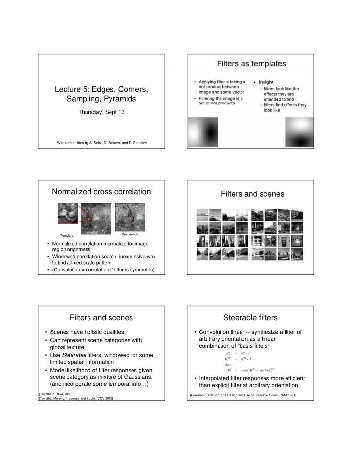
Lecture 5: Edges, Corners, Sampling, Pyramids Thursday, Sept 13 - PDF document

Lecture 5: Edges, Corners, Sampling, Pyramids Thursday, Sept 13 With some slides by S. Seitz, D. Frolova, and D. Simakov Normalized cross correlation Filters and scenes Best match Template • Normalized correlation: normalize for image region brightness • Windowed correlation search: inexpensive way to find a fixed scale pattern • (Convolution = correlation if filter is symmetric) Filters and scenes Steerable filters • Scenes have holistic qualities • Convolution linear -- synthesize a filter of arbitrary orientation as a linear • Can represent scene categories with combination of “basis filters” global texture • Use Steerable filters, windowed for some limited spatial information • Model likelihood of filter responses given scene category as mixture of Gaussians, • Interpolated filter responses more efficient (and incorporate some temporal info…) than explicit filter at arbitrary orientation [Torralba & Oliva, 2003] [Freeman & Adelson, The Design and Use of Steerable Filters, PAMI 1991] [Torralba, Murphy, Freeman, and Rubin, ICCV 2003]

Steerable filters Freeman & Adelson, 1991 Probability of the = scene given global Basis filters for derivative of Gaussian features = [Torralba, Murphy, Freeman, and Rubin, ICCV 2003] Contextual priors • Use scene recognition � predict objects present • For object(s) likely to be present, predict locations based on similarity to previous images with the same place and that object [Torralba, Murphy, Freeman, and Rubin, ICCV 2003] Scene category Blue solid circle: recognition with temporal info Specific place Black hollow circle: instantaneous (black=right, red=wrong) recognition using global feature only Cross: true location [Torralba, Murphy, Freeman, and Rubin, ICCV 2003]

Image gradient Effects of noise The gradient of an image: Consider a single row or column of the image • Plotting intensity as a function of position gives a signal The gradient points in the direction of most rapid change in intensity The gradient direction (orientation of edge normal) is given by: The edge strength is given by the gradient magnitude Where is the edge? Slide credit S. Seitz Solution: smooth first Derivative theorem of convolution This saves us one operation: Where is the edge? Look for peaks in Laplacian of Gaussian 2D edge detection filters Consider Laplacian of Gaussian Gaussian derivative of Gaussian Laplacian of Gaussian operator • is the Laplacian operator: Where is the edge? Zero-crossings of bottom graph

The Canny edge detector The Canny edge detector original image (Lena) norm of the gradient The Canny edge detector Non-maximum suppression Check if pixel is local maximum along gradient direction, select single max across width of the edge thresholding • requires checking interpolated pixels p and r The Canny edge detector Predicting the next edge point Assume the marked point is an edge point. Then we construct the tangent to the edge curve (which is normal to the gradient at that point) and use this to predict the next points (here either r or s). thinning (non-maximum suppression) (Forsyth & Ponce)

Hysteresis Thresholding Edge detection by subtraction Reduces the probability of false contours and fragmented edges Given result of non-maximum suppression: For all edge points that remain, - locate next unvisited pixel where intensity > t high - start from that point, follow chains along edge and add points where intensity < t low original Edge detection by subtraction Edge detection by subtraction Why does this work? smoothed – original smoothed (5x5 Gaussian) (scaled by 4, offset +128) Gaussian - image filter Causes of edges Gaussian delta function If the goal is image understanding, what do we want from an edge detector? Laplacian of Gaussian Adapted from C. Rasmussen

Human- Learning good boundaries marked segment boundaries • Use ground truth (human-labeled) boundaries in natural images to learn good features • Supervised learning to optimize cue integration, filter scales, select feature types Work by D. Martin and C. Fowlkes and D. Tal and J. Malik, Berkeley Segmentation Benchmark, 2001 [D. Martin et al. PAMI 2004] What features are responsible What features are responsible for perceived edges? for perceived edges? Feature profiles (oriented energy, brightness, color, and texture gradients) along the patch’s horizontal diameter [D. Martin et al. PAMI 2004] Learning good boundaries Original Human-labeled Boundary detection [D. Martin et al. PAMI 2004] Berkeley Segmentation Database, D. Martin and C. Fowlkes and D. Tal and J. Malik

Edge detection and corners • Partial derivative estimates in x and y fail to capture corners Why do we care about corners? [D. Martin et al. PAMI 2004] Case study: panorama stitching How do we build panorama? • We need to match (align) images [Brown, Szeliski, and Winder, CVPR 2005] [Slide credit: Darya Frolova and Denis Simakov] Matching with Features Matching with Features • Detect feature points in both images • Detect feature points in both images • Find corresponding pairs

Matching with Features Matching with Features • Detect feature points in both images • Problem 1: • Find corresponding pairs – Detect the same point independently in both • Use these pairs to align images images no chance to match! We need a repeatable detector Matching with Features Corner detection as an interest operator • (Problem 2: • We should easily recognize the point by looking through a small window – For each point correctly recognize the • Shifting a window in any direction should corresponding one) give a large change in intensity ? We need a reliable and distinctive descriptor More on this aspect later! Corner detection as an interest operator Corner Detection M is a 2 × 2 matrix computed from image derivatives: ⎡ ⎤ 2 I I I Gradient with ∑ = x x y ⎢ ⎥ M w x y ( , ) respect to x, ⎢ I I I 2 ⎥ times gradient ⎣ ⎦ x y , x y y with respect to y Sum over image region – area “flat” region: “edge”: “corner”: we are checking for corner no change in no change along significant change all directions the edge direction in all directions C.Harris, M.Stephens. “A Combined Corner and Edge Detector”. 1988

Corner Detection Corner Detection Eigenvectors of M: encode edge directions λ 2 Classification of “Edge” λ 2 >> λ 1 Eigenvalues of M: encode edge strength image points using “Corner” eigenvalues of M : λ 1 and λ 2 are large, λ 1 ~ λ 2 ; λ 1 , λ 2 – eigenvalues of M E increases in all direction of the fastest change directions direction of the slowest change λ max λ min λ 1 and λ 2 are small; “Edge” E is almost constant “Flat” λ 1 >> λ 2 in all directions region λ 1 Harris Corner Detector Harris Corner Detector Measure of corner response: λ 2 “Edge” “Corner” • R depends only on R < 0 ( ) = − 2 R M k M det trace eigenvalues of M Avoid computing • R is large for a corner R > 0 eigenvalues • R is negative with large = λ λ M themselves. det 1 2 magnitude for an edge = λ + λ trace M • | R | is small for a flat 1 2 region “Flat” “Edge” ( k – empirical constant, k = 0.04-0.06) |R| small R < 0 λ 1 Harris Detector: Workflow Harris Corner Detector • The Algorithm: – Find points with large corner response function R ( R > threshold) – Take the points of local maxima of R

Harris Detector: Workflow Harris Detector: Workflow Compute corner response R Find points with large corner response: R> threshold Harris Detector: Workflow Harris Detector: Workflow Take only the points of local maxima of R Harris Detector: Some Properties Harris Detector: Some Properties • Rotation invariance • Not invariant to image scale ! Ellipse rotates but its shape (i.e. eigenvalues) remains the same All points will be Corner ! Corner response R is invariant to image rotation classified as edges More on interest operators/descriptors with invariance properties later.

This image is too big to fit on the screen. How can we reduce it? How to generate a half- sized version? Image sub-sampling Image sub-sampling 1/8 1/4 Throw away every other row and 1/2 1/4 (2x zoom) 1/8 (4x zoom) column to create a 1/2 size image - called image sub-sampling Slide credit: S. Seitz Sampling Undersampling • Continuous function � discrete set of • Information lost values Figure credit: S. Marschner

Undersampling Undersampling • Looks just like lower frequency signal! • Looks like higher frequency signal! Aliasing : higher frequency information can appear as lower frequency information Undersampling Aliasing Good sampling Bad sampling Aliasing in video Aliasing Input signal: Matlab output: x = 0:.05:5; imagesc(sin((2.^x).*x)) Not enough samples Slide credit: S. Seitz