Fractional Gaussian Noise, Fractional Gaussian Noise, Subdiffusion and Stochastic and Stochastic Subdiffusion Networks in Biophysics Networks in Biophysics Samuel Kou Department of Statistics Harvard University
Single-Molecule Experiments � Statistics & probability experienced fundamental change in the past 20 years � Biophysics & chemistry also witnessed dramatic progress: single-molecule experiments � Using nanotechnology, scientists can study biological processes on a single-molecule basis (eg. enzymatic kinetics, protein/DNA dynamics) “Seeing images of single atoms is a religious experience” --- Richard Feynman
New Aspects for Scientific Discovery � Can measure molecular properties individually , instead of inferring from population statistics � If the reaction/kinetic time is slow, ensemble experiments become almost impossible due to the difficulty of synchronization � Single-molecule trajectory provides detailed dynamic information � Understanding the dynamics of individual is essential to unlock their biofunctions
Statistical & Probabilistic Challenges Statistical & Probabilistic Challenges � Require new stochastic modeling Subdiffusion Enzymatic reaction � Data are noisier, and efficient inference methodology is needed
Brownian diffusion � Since Einstein's 1905 paper, the theory of Brownian diffusion has revolutionized not only natural sciences but also social sciences. � Brownian motion described by Langevin equation dv = ζ − + m t v F ( t ) t dt where F ( t ) is white noise process satisfying ′ ′ = ζ ⋅ δ − E F t F t k T t t { ( ) ( )} ( ) B by fluctuation-dissipation theorem. � Solution: Ornstein-Uhlenbeck process v ( t ) Gaussian t � Displacement (location) = x t ∫ v s ds ( ) ( ) 0 k T ∼ E x t 2 B t t { ( ) } 2 , for large ζ --- Corner stone for statistical mechanics
Subdiffusion � Brownian diffusion, however, cannot explain so called subdiffusion: α ∝ < α < E x t 2 t { ( ) } , 0 1 � Distance fluctuation within a single protein molecule (Yang et al . 2003, Science ; Min et al . 2005, Physical Review Letters ). � Need tools beyond Langevin equation and BM.
Single-molecule fluorescence experiment on protein complex � Yang et al. (2003, Science ) studied a protein-enzyme complex Fre , catalyzes the reduction of flavin � Fre contains two substructures: a flavin adenine dinucleotide (FAD) and a tyrosine (Tyr). � Fluorescence lifetime of FAD varies Tyr due to distance fluctuation � Relationship between fluorescence FAD lifetime and distance − β + X X γ − = − ( ) 1 t k e 1 ( ) [ eq t ] 0
− − ∆ γ ∆ γ Autocorrelation function E 1 1 t { ( 0 ) ( )} ∆ γ − = γ − − γ − 1 t 1 t E 1 t ( ) ( ) { ( )} 0.06 • Need tools beyond Langevin equation and BM. 0.04 C γ ( t ) • The model: Generalized Langevin equation with 0.02 fractional Gaussian noise (GLE with fGn). 0.00 0.001 0.01 0.1 1 10 100 1000 time (second)
Generalized Langevin Equation with fGn dv = ζ − + � Langevin equation m t v F ( t ) t dt dv t ∫ ∞ = − ζ − + m t v K t u du G � Generalized Langevin equation ( ) , u t dt − � Fluctuation-dissipation theorem links memory kernel K ( t ) with fluctuating force = ζ ⋅ − E G G k T K t s { } ( ) t s B � Key question: How to introduce the noise structure? � Understand the white noise: White noise is the F = derivative of the Wiener process d B t t dt � B ( t ) is the unique process: (i) Gaussian, (ii) independent increment, (iii) stationary increment, (iv) self-similar
� Natural generalization: (i) Gaussian (ii) stationary increment (iii) self-similar. � The ONLY candidate fBM B ( H ) ( t ) , 0 < H < 1 = H E B ( ) , and covariance function { } 0 t H H H 2 2 2 = + − − ≥ H H E B ( ) B ( ) t s t s t s { } ( ) / 2 for , 0 . t s when H = 1/2, reduces to B ( t ). H ( ) = dB H � Fractional Gaussian noise : F ( ) t ( ) t dt Gaussian & stationary. � Memory kernel = H H K t E F ( ) F ( ) t ( ) { ( 0 ) ( )} H − = − ≠ H H H t 2 2 t ( 2 1 ) | | , for 0 � Spectral density = ∫ ~ ∞ ϖ − ϖ = Γ + π ϖ it H K e K t dt H H 1 2 ( ) ( ) ( 2 1 ) sin( ) | | H H − ∞
Toward subdiffusion � Applying Fourier transform on dv t ∫ ∞ ( H = − ζ − + ) m t v K t u du F ( ) , u H t dt − v ( t ) Gaussian E { v ( t )} = 0, 1 ∞ ~ ∫ = = ϖ ϖ ϖ it C t E v v t e C d ( ) { ( 0 ) ( )} ( ) π − ∞ 2 ~ ζ ϖ k T K ~ ( ) ϖ = C B H ( ) ~ 2 + ζ ϖ − ϖ K i m ( ) H ( ) � For displacement = t X t v s ds ∫ ( ) 0 t t ∫ ∫ = E X t 2 E v s v u du ds { ( ) } { ( ) ( )} 0 0 π k T H 2 sin( 2 ) − − H ∝ H E X t 2 B t 2 2 t 2 2 { ( ) } ~ ζ π − − H H H ( 2 1 )( 2 2 ) � H > 1/2 leads to subdiffusion!
Harmonic potential dv t ∫ ∞ ( H = − ζ − + ) � GLE: m t v K t u du F ( ) , u H t dt − � For external field U ( x ) , changes to t ∫ ∞ & & & ′ = − ζ − − + H m X t X u K t u du U X F ( ) t ( ) ( ) ( ) ( ) ( ) H t − & & = t = dv t where , . ( ) X t v s ds X t ∫ ( ) ( ) ( ) dt 0 = ω For harmonic potential U x m x 2 2 1 ( ) 2 t ∫ ∞ & & & = − ζ − − ω + H m X t X u K t u du m 2 X t F ( ) t ( ) ( ) ( ) ( ) ( ) H − � Fourier method gives E { X ( t ) X ( s )}, E { X ( t ) v ( s )} Overdamped condition � Acceleration negligible, GLE reads t ∫ ∞ & ω = − ζ − + H m 2 X t X u K t u du F ( ) t ( ) ( ) ( ) ( ) H −
t ∫ ∞ & ω = − ζ − + H m 2 X t X u K t u du F ( ) t ( ) ( ) ( ) ( ) H − � Solution: X ( t ) stationary Gaussian E { X ( t )}=0 = C t E X X t ( ) { ( 0 ) ( )} xx ω k T m 2 − = − H B E t 2 2 ( ) − H ω ζ Γ + 2 2 m H 2 ( 2 1 ) ∞ = ∑ Γ α + k E z z k where ( ) / ( 1 ) α = k 0 � For all H , k T = = C E X X B ( 0 ) { ( 0 ) ( 0 )} xx ω m 2 the thermal equilibrium value. � For H = 1/2, recovers the Brownian diffusion result k T 2 ω − m t 2 = = C t E X X t B e ζ ( ) { ( 0 ) ( )} xx ω m 2
The Hamiltonian for GLE with fGn � GLE with fGn can be derived from the interaction between a particle and a harmonic oscillator heat bath. 1 1 = + ω H s mv 2 m 2 x 2 � Start from system Hamiltonian 2 2 p 2 1 = + ω = m 2 x 2 p mv , and the heat bath Hamiltonian m 2 2 ⎛ ⎞ γ p 2 = ∑ 1 ⎜ ⎟ j j + ω − H m 2 q x 2 ( ) ⎜ ⎟ B b j j ω m 2 2 2 ⎝ ⎠ j b j where m b the media molecule mass, ω j individual frequency, and γ j coupling strength of j th oscillator. � Equation of motion for H s + H B ∂ ∂ dx dp = + = − + H H H H ( ), ( ) s B s B ∂ ∂ dt p dt x dq ∂ dp ∂ j = + j = − + H H H H ( ), ( ) s B s B ∂ ∂ dt p dt q j j
� Solve it. Leads to (i) GLE t ∫ ∞ & & & = − ζ − − ω + m X t X u K t u du m 2 X t F t ( ) ( ) ( ) ( ) ( ) − where γ 2 γ ϖ 2 ( ) ∑ ∫ j = ω = ϖ ϖ ϖ K t m t m t g d ( ) cos cos( ) ( ) b j b ω ϖ 2 2 j j γ γ ∑ ∑ j j = γ − ω + ω F t m q x t p t ( ) ( ( 0 ) ( 0 )) cos( ) ( 0 ) sin( ) b j j j j j ω ω 2 j j j j and (ii) the fluctuation-dissipation theorem = ζ ⋅ − E F F k T K t s { } ( ) t s B � Furthermore, if we take 2 g 1 Γ 2 H 1 sin H | | 3 − 2 H fGn memory kernel K t H 2 H − 1 t 2 H − 2
Back to experiment Fluorescence lifetime of FAD depends on the distance between Tyr FAD and Tyr − β + X X γ − = − ( ) FAD 1 t k e 1 ( ) [ eq t ] 0 Model X ( t ) by GLE with fGn under harmonic potential easy calculation of lifetime autocorrelation β + β 2 − − X C β 2 γ γ = − 2 ( 0 ) C t Cov 1 1 t k 2 e e ( ) eq xx { ( 0 ), ( )} ( 1 ) xx 0
Fitting experimental autocorrelation 0.06 ζ k B T 2 β 2 H ω 2 ω m m 0.04 C γ ( t ) 0.74 0.40 0.81 0.02 0.00 0.001 0.01 0.1 1 10 100 1000 Kou and Xie, Phys. Rev. Lett. , 93 , time (second) 180603 (2004).
Higher order autocorrelation functions − − − δγ = γ − 〈 γ 〉 1 t 1 t 1 t ( ) : ( ) ( ) 1.0 〈δγ −1 (0) δγ −1 (t) δγ −1 (2t) δγ −1 (3t) 〉 〈δγ −1 (0) δγ −1 (t) δγ −1 (2t) 〉 5 〈γ −1 〉 3 〈γ −1 〉 3 0.8 4 Three-point Four-point 0.6 3 0.4 2 0.2 1 0.0 0 0.001 0.01 0.1 1 10 0.001 0.01 0.1 1 10 t (sec) t (sec) ζ k B T 2 β 2 H Same parameters: ω 2 ω m m 0.74 0.40 0.81
Recommend
More recommend
Unleash a World of Digital Possibilities—Browse, Share, and Explore Content Without Boundaries