Fractional Gaussian Fields for Modeling and Rendering of - PowerPoint PPT Presentation

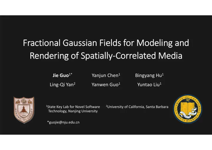
Fractional Gaussian Fields for Modeling and Rendering of Spatially‐Correlated Media Jie Guo 1* Yanjun Chen 1 Bingyang Hu 1 Ling‐Qi Yan 2 Yanwen Guo 1 Yuntao Liu 1 1 State Key Lab for Novel Software 2 University of California, Santa Barbara Technology, Nanjing University *guojie@nju.edu.cn

Participating Media stanschaap.com

Participating Media videoblocks.com

Participating Media

Participating Media scattering

Participating Media absorption

Participating Media Independent Scattering Approximation Classical Radiative Transport Equation

Related Work (But, a lot of works have observed correlations in particle distribution)

Related Work

Related Work [Meng et al. 2015] [Müller et al. 2016] [Bitterli et al. 2018] [Jarabo et al. 2018]

Related Work [Meng et al. 2015] [Müller et al. 2016] [Bitterli et al. 2018] [Jarabo et al. 2018]

Our method  General media  Heterogeneity  Long‐range correlations

Spatially‐Correlated Media Uncorrelated Media Correlated Media Uncorrelated Media

Spatially‐Correlated Media Correlated Media Uncorrelated Media

Spatially‐Correlated Media 𝜏 � 𝒚 𝒛 𝜕 � 𝜏 � 𝑢 � �� � 𝑓 �� 𝒚,� � Transmittance : 𝑈 𝒚, 𝒛 � 𝑓 � � � � 𝒚��� � 𝜏 � 𝒚 � 𝜏 � 𝒚 � 𝜏 � 𝒚 Extinction field :

Spatially‐Correlated Media 𝜏 � 𝒚 𝒛 𝜕 � 𝜏 � 𝑢 � �� � 𝑓 �� 𝒚,� � Transmittance : 𝑈 𝒚, 𝒛 � 𝑓 � � � � 𝒚��� � 𝜏 � 𝒚 � 𝜏 � 𝒚 � 𝜏 � 𝒚 Extinction field : We model 𝜏 � as a Fractional Gaussian Field (FGF)

Fractional Gaussian Fields Random field A collection of random variables: 𝑌 � 𝑌 𝑢, 𝜕 , 𝑢 ∈ ℝ � , 𝜕 ∈ Ω 𝑢 𝜕

Fractional Gaussian Fields Random field A collection of random variables: 𝑌 � 𝑌 𝑢, 𝜕 , 𝑢 ∈ ℝ � , 𝜕 ∈ Ω 𝑌 𝑢 � ,· 𝑢 𝜕

Fractional Gaussian Fields Random field A collection of random variables: 𝑌 � 𝑌 𝑢, 𝜕 , 𝑢 ∈ ℝ � , 𝜕 ∈ Ω 𝑢 𝑌 ·, 𝜕 � realization 𝜕

Fractional Gaussian Fields Random field A collection of random variables: 𝑌 � 𝑌 𝑢, 𝜕 , 𝑢 ∈ ℝ � , 𝜕 ∈ Ω Gaussian (random) field A collection of Gaussian‐distributed random variables. White Noise

Fractional Gaussian Fields Then what is “ fractional ”? Let 𝐽 be the integral operator 𝐽 � 1 � 𝑦 � /2 𝐽 1 � 𝑦 𝐽 𝑦 � ? 𝐽 � 𝑦 � ? , 𝑏 � 0

Fractional Gaussian Fields Then what is “ fractional ”? Let 𝐽 be the integral operator 𝐽 � 1 � 𝑦 � /2 𝐽 1 � 𝑦 𝐽 𝑦 � ? 𝐽 � 𝑦 � ? , 𝑏 � 0

Fractional Gaussian Fields With the fractional integral operator 𝐽 � �.� [ ] White Noise

Fractional Gaussian Fields With the fractional integral operator 𝐽 � �.� [ ] White Noise

Fractional Gaussian Fields With the fractional integral operator 𝐽 � �.� [ ] White Noise

Fractional Gaussian Fields Fractional Gaussian Fields

Fractional Gaussian Fields �� 𝑒 ‐dimensional FGF: � 𝑋 : white noise fractional Laplacian 𝑡 � 0 white noise The FGF family 𝑡 � 1, 𝑒 � 1 Brownian motion 1 2 � 𝑡 � 3 fractional Brownian motion 2 , 𝑒 � 1 (fBm)

Fractional Gaussian Fields �� 𝑒 ‐dimensional FGF: � 𝑋 : white noise � Hurst parameter 𝐼 � 𝑡 � � 𝐼 Correlation

Autocovariance Function �� 𝑒 ‐dimensional FGF: � 𝑋 : white noise Autocovariance function of pink noise: 𝐷 𝐼, 𝑒 Scaling term 𝑇 � Power spectral density of white noise

Autocovariance Function �� 𝑒 ‐dimensional FGF: � 𝑋 : white noise Autocovariance function of k‐fBm:

Autocovariance Function covariance matrix (1D) Pink noise (H<0) k‐fBm (H>0)

Autocovariance Function covariance matrix (1D) Pink noise Long‐range correlation k‐fBm

2D Fractional Gaussian Fields

2D Fractional Gaussian Fields 𝐼 Correlation Aggregates

Extinction Field We model 𝜏 � as a FGF : � � � var�𝜏 � 𝒚 � �? Macro‐scale: Constant Micro‐scale: FGF Fixing 𝒚 , 𝜏 � 𝒚 is a random variable with mean 𝜏 � and its variance is controlled by the FGF

Extinction Field We model 𝜏 � as a FGF : � � � � 𝒚��� � �� � 𝒚,� The line‐averaged extinction 𝜏 � 𝒚 � � � is a � � Gaussian‐distributed random variable. � � var 𝜏 � � 1 � � 1 𝜐 𝒚, 𝑢 � � 𝜐 𝒚, 𝑢 𝑢 � � � cov 𝒚 � , 𝒚 �� d𝑢 � d𝑢 �� 𝑢 � � � autocovariance function of the FGF

Extinction Field Pink noise (H<0) � � var 𝜏 � � 1 � � 1 𝜐 𝒚, 𝑢 � � 𝜐 𝒚, 𝑢 𝑢 � � � cov 𝒚 � , 𝒚 �� d𝑢 � d𝑢 �� 𝑢 � � �

Extinction Field k‐fBm (H>0) � � var 𝜏 � � 1 � � 1 𝜐 𝒚, 𝑢 � � 𝜐 𝒚, 𝑢 𝑢 � � � cov 𝒚 � , 𝒚 �� d𝑢 � d𝑢 �� 𝑢 � � �

Extinction Field Numerical verification:

Extinction Field Numerical verification: One‐point scale‐independence Pink noise k‐fBm

Extinction Field The variance of 𝜏 � 𝒚 : White noise Pink noise K‐fBm

Transmittance Ensemble‐averaged transmittance � � 𝑓 ��� � � � 𝑓 ��� � 𝑞𝑒𝑔 𝜏 � d𝜏 � Tr 𝑢 �

Transmittance Ensemble‐averaged transmittance � � 𝑓 ��� � � � 𝑓 ��� � 𝑞𝑒𝑔 𝜏 � d𝜏 � Tr 𝑢 � characteristic function 𝜒 � � 𝐣𝑢 𝜏 � � 𝜏 � 𝜏 � ~ Γ� , � Use gamma distribution for non‐negative extinction var 𝜏 � var 𝜏 �

Transmittance Ensemble‐averaged transmittance � � 𝑓 ��� � � � 𝑓 ��� � 𝑞𝑒𝑔 𝜏 � d𝜏 � Tr 𝑢 �

Transmittance Transparent

Transmittance 𝐼 � �0.2 𝐼 � 0.5 𝐼 � 0.8

Rendering Techniques Energy‐Conserving Volumetric Rendering Equation Transport kernel:

Results

Short‐range correlations Long‐range correlations

Low density

Comparing to the GBE [Jarabo et al. 2018]

Comparing to the Bitterli model [Bitterli et al. 2018]

Uncorrelated media

Correlated media

Conclusion  A mathematical tool for physically‐based modeling spatial correlations in random media.  Using k‐th order fBm to generate long‐range correlations.  The usage of the non‐exponential transmittance functions in an energy‐ conserving RTE framework.

Thank you! Q&A