Forecasting the 2012 Presidential Election from History and the - - PowerPoint PPT Presentation

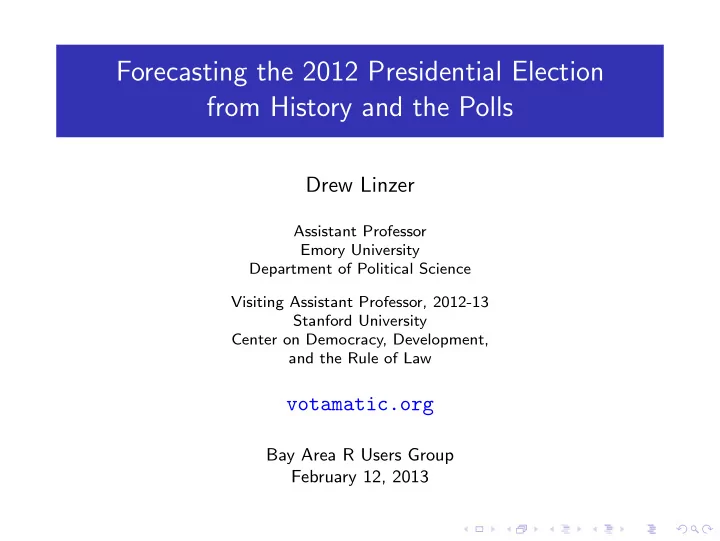
Forecasting the 2012 Presidential Election from History and the Polls

Drew Linzer

Assistant Professor Emory University Department of Political Science Visiting Assistant Professor, 2012-13 Stanford University Center on Democracy, Development, and the Rule of Law

votamatic.org

Bay Area R Users Group February 12, 2013

The 2012 Presidential Election: Obama 332–Romney 206

The 2012 Presidential Election: Obama 332–Romney 206

But also: Nerds 1–Pundits 0

The 2012 Presidential Election: Obama 332–Romney 206

But also: Nerds 1–Pundits 0 Analyst forecasts based on history and the polls

Drew Linzer, Emory University 332-206 Simon Jackman, Stanford University 332-206 Josh Putnam, Davidson College 332-206 Nate Silver, New York Times 332-206 Sam Wang, Princeton University 303-235

Pundit forecasts based on intuition and gut instinct

Karl Rove, Fox News 259-279 Newt Gingrich, Republican politician 223-315 Michael Barone, Washington Examiner 223-315 George Will, Washington Post 217-321 Steve Forbes, Forbes Magazine 217-321

What we want: Accurate forecasts as early as possible

The problem:

• The data that are available early aren’t accurate:

Fundamental variables (economy, approval, incumbency)

• The data that are accurate aren’t available early:

Late-campaign state-level public opinion polls

• The polls contain sampling error, house effects, and most

states aren’t even polled on most days

What we want: Accurate forecasts as early as possible

The problem:

• The data that are available early aren’t accurate:

Fundamental variables (economy, approval, incumbency)

• The data that are accurate aren’t available early:

Late-campaign state-level public opinion polls

• The polls contain sampling error, house effects, and most

states aren’t even polled on most days

The solution:

• A statistical model that uses what we know about presidential

campaigns to update forecasts from the polls in real time

What we want: Accurate forecasts as early as possible

The problem:

• The data that are available early aren’t accurate:

Fundamental variables (economy, approval, incumbency)

• The data that are accurate aren’t available early:

Late-campaign state-level public opinion polls

• The polls contain sampling error, house effects, and most

states aren’t even polled on most days

The solution:

• A statistical model that uses what we know about presidential

campaigns to update forecasts from the polls in real time

What do we know?

• 1. The fundamentals predict national outcomes, noisily

Election year economic growth

Source: U.S. Bureau of Economic Analysis

• 1. The fundamentals predict national outcomes, noisily

Presidential approval, June

Source: Gallup

• 2. States vote outcomes swing (mostly) in tandem

Source: New York Times

• 3. Polls are accurate on Election Day; maybe not before

May Jul Sep Nov 40 45 50 55 60

Florida: Obama, 2008

Obama vote share

Actual

• utcome

Source: HuffPost-Pollster

• 4. Voter preferences evolve in similar ways across states

May Jul Sep Nov 40 45 50 55 60

Florida: Obama, 2008

Obama vote share May Jul Sep Nov 40 45 50 55 60

Virginia: Obama, 2008

Obama vote share May Jul Sep Nov 40 45 50 55 60

Ohio: Obama, 2008

Obama vote share May Jul Sep Nov 40 45 50 55 60

Colorado: Obama, 2008

Obama vote share

Source: HuffPost-Pollster

• 5. Voters have short term reactions to big campaign events

Source: Tom Holbrook, UW-Milwaukee

All together: A forecasting model that learns from the polls

Publicly available state polls during the campaign

Months prior to Election Day Cumulative number of polls fielded 12 11 10 9 8 7 6 5 4 3 2 1 500 1000 1500 2000

2008 2012

Forecasts weight fundamentals ← → Forecasts weight polls

Source: HuffPost-Pollster

First, create a baseline forecast of each state outcome

Abramowitz Time-for-Change regression makes a national forecast: Incumbent vote share = 51.5 + 0.6 Q2 GDP growth + 0.1 June net approval − 4.3 In office two+ terms

First, create a baseline forecast of each state outcome

Abramowitz Time-for-Change regression makes a national forecast: Incumbent vote share = 51.5 + 0.6 Q2 GDP growth + 0.1 June net approval − 4.3 In office two+ terms Predicted Obama 2012 vote = 51.5 + 0.6 (1.3) + 0.1 (-0.8) − 4.3 (0)

First, create a baseline forecast of each state outcome

Abramowitz Time-for-Change regression makes a national forecast: Incumbent vote share = 51.5 + 0.6 Q2 GDP growth + 0.1 June net approval − 4.3 In office two+ terms Predicted Obama 2012 vote = 51.5 + 0.6 (1.3) + 0.1 (-0.8) − 4.3 (0) Predicted Obama 2012 vote = 52.2%

First, create a baseline forecast of each state outcome

Abramowitz Time-for-Change regression makes a national forecast: Incumbent vote share = 51.5 + 0.6 Q2 GDP growth + 0.1 June net approval − 4.3 In office two+ terms Predicted Obama 2012 vote = 51.5 + 0.6 (1.3) + 0.1 (-0.8) − 4.3 (0) Predicted Obama 2012 vote = 52.2% Use uniform swing assumption to translate to the state level: Subtract 1.5% for Obama from his 2008 state vote shares Make this a Bayesian prior over the final state outcomes

Combine polls across days and states to estimate trends

States with many polls States with fewer polls

• May

Jun Jul Aug Sep Oct Nov 44 46 48 50 52 54 56

Florida: Obama, 2012

Obama vote share

• May

Jun Jul Aug Sep Oct Nov 44 46 48 50 52 54 56

Oregon: Obama, 2012

Obama vote share

Combine with baseline forecasts to guide future projections

Random walk (no)

• May

Jun Jul Aug Sep Oct Nov 44 46 48 50 52 54 56

Florida: Obama, 2012

Obama vote share

Combine with baseline forecasts to guide future projections

Random walk (no) Mean reversion

• May

Jun Jul Aug Sep Oct Nov 44 46 48 50 52 54 56

Florida: Obama, 2012

Obama vote share

• May

Jun Jul Aug Sep Oct Nov 44 46 48 50 52 54 56

Florida: Obama, 2012

Obama vote share

Forecasts compromise between history and the polls

A dynamic Bayesian forecasting model

Model specification

yk ∼ Binomial(πi[k]j[k], nk)

Number of people preferring Democrat in survey k, in state i, on day j

πij = logit−1(βij + δj)

Proportion reporting support for the Democrat in state i on day j National effects: δj State components: βij Election forecasts: ˆ πiJ

Priors

βiJ ∼ N(logit(hi), τi)

Informative prior on Election Day, using historical predictions hi, precisions τi

δJ ≡ 0

Polls assumed accurate, on average

βij ∼ N(βi(j+1), σ2

β)

Reverse random walk, states

δj ∼ N(δ(j+1), σ2

δ)

Reverse random walk, national

A dynamic Bayesian forecasting model

Model specification

yk ∼ Binomial(πi[k]j[k], nk)

Number of people preferring Democrat in survey k, in state i, on day j

πij = logit−1(βij + δj)

Proportion reporting support for the Democrat in state i on day j National effects: δj State components: βij Election forecasts: ˆ πiJ

Priors

βiJ ∼ N(logit(hi), τi)

Informative prior on Election Day, using historical predictions hi, precisions τi

δJ ≡ 0

Polls assumed accurate, on average

βij ∼ N(βi(j+1), σ2

β)

Reverse random walk, states

δj ∼ N(δ(j+1), σ2

δ)

Reverse random walk, national

Estimated for all states simultaneously

Results: Anchoring to the fundamentals stabilizes forecasts

• ●
• ● ●
• ● ●
• ●● ●
• ● ● ●●●
• ●●● ●
• ●●● ●●●
• Jul

Aug Sep Oct Nov 40 45 50 55 60

Florida: Obama forecasts, 2012

Obama vote share

Shaded area indicates 95% uncertainty

Results: Anchoring to the fundamentals stabilizes forecasts

Electoral Votes

Jul Aug Sep Oct Nov 150 200 250 300 350 400

OBAMA 332 ROMNEY 206

There were almost no surprises in 2012

On Election Day, average error = 1.7% Why didn’t the model do more?

There were almost no surprises in 2012

On Election Day, average error = 1.7%

There were almost no surprises in 2012

On Election Day, average error = 1.7% Why didn’t the model improve forecasts by more?

The fundamentals and uniform swing were right on target

• 30

40 50 60 70 30 40 50 60 70

State election outcomes

2008 Obama vote 2012 Obama vote

AL AK AZ AR CA CO CT DE FL GA HI ID IL IN IA KS KY LA ME MD MA MI MN MS MO MT NE NV NH NJ NM NY NC ND OH OK OR PA RI SC SD TN TX UT VT VA WA WV WI WY

2012=2008 line

Aggregate preferences were very stable

Percent supporting: Obama Romney

Could the model have done better? Yes

• 20

40 60 80 100 −6 −4 −2 2 4 6 Difference between actual and predicted vote outcomes Number of polls after May 1, 2012 Election Day forecast error

AL AK AZ AR CA CO CT DE FL GA HI ID IL IN IA KS KY LA ME MD MA MI MN MS MO MT NE NV NH NJ NM NY NC ND OH OK OR PA RI SC SD TN TX UT VT VA WA WV WI WY

↑ Obama performed

better than expected

↓ Romney performed

better than expected

Forecasting is only one of many applications for the model

1 Who’s going to win? 2 Which states are going to be competitive? 3 What are current voter preferences in each state? 4 How much does opinion fluctuate during a campaign? 5 What effect does campaign news/activity have on opinion? 6 Are changes in preferences primarily national or local? 7 How useful are historical factors vs. polls for forecasting? 8 How early can accurate forecasts be made? 9 Were some survey firms biased in one direction or the other?

House effects (biases) were evident during the campaign

Much more at votamatic.org drew@votamatic.org @DrewLinzer