Fixing the Gaussian Blur: the Bilateral Filter Sylvain Paris MIT - PowerPoint PPT Presentation
A Gentle Introduction A Gentle Introduction to Bilateral Filtering to Bilateral Filtering and its Applications and its Applications Fixing the Gaussian Blur: the Bilateral Filter Sylvain Paris MIT CSAIL Blur Comes from Blur Comes
A Gentle Introduction A Gentle Introduction to Bilateral Filtering to Bilateral Filtering and its Applications and its Applications “Fixing the Gaussian Blur”: the Bilateral Filter Sylvain Paris – MIT CSAIL
Blur Comes from Blur Comes from Averaging across Edges Averaging across Edges * output input * * Same Gaussian kernel everywhere.
Bilateral Filter Bilateral Filter [Aurich 95, Smith 97, Tomasi 98] No Averaging across Edges No Averaging across Edges * output input * * The kernel shape depends on the image content.
Bilateral Filter Definition: Bilateral Filter Definition: an Additional Edge Term an Additional Edge Term Same idea: weighted average of pixels . new not new new ( ) 1 ( ) ∑ = − − [ ] || || | | p q BF I G G I I I σ σ p p q q s r W ∈ q S p normalization space weight range weight factor I
Illustration a 1D Image Illustration a 1D Image • 1D image = line of pixels • Better visualized as a plot pixel intensity pixel position
Gaussian Blur and Bilateral Filter Gaussian Blur and Bilateral Filter Gaussian blur p ( ) ∑ = − [ ] || || p q GB I G I q σ p q ∈ q S space space Bilateral filter [Aurich 95, Smith 97, Tomasi 98] p ( ) 1 ( ) range ∑ = − − [ ] || || | | BF I G p q G I I I σ σ p p q q s r W q ∈ q S p space range normalization space
Bilateral Filter on a Height Field Bilateral Filter on a Height Field ( ) 1 ( ) ∑ = − − [ ] || || | | p q BF I G G I I I σ σ p p q q s r W ∈ q S p p p p p q q output input reproduced from [Durand 02]
Space and Range Parameters Space and Range Parameters ( ) 1 ( ) ∑ = − − [ ] || || | | BF I G p q G I I I σ σ p p q q s r W ∈ q S p • space σ s : spatial extent of the kernel, size of the considered neighborhood. • range σ r : “minimum” amplitude of an edge
Influence of Pixels Influence of Pixels Only pixels close in space and in range are considered. space range p p
Exploring the Parameter Space Exploring the Parameter Space σ r = ∞ σ r = 0.1 σ r = 0.25 (Gaussian blur) input σ s = 2 σ s = 6 σ s = 18
Varying the Range Parameter Varying the Range Parameter σ r = ∞ σ r = 0.1 σ r = 0.25 (Gaussian blur) input σ s = 2 σ s = 6 σ s = 18
input
σ r = 0.1
σ r = 0.25
σ r = ∞ (Gaussian blur)
Varying the Space Parameter Varying the Space Parameter σ r = ∞ σ r = 0.1 σ r = 0.25 (Gaussian blur) input σ s = 2 σ s = 6 σ s = 18
input
σ s = 2
σ s = 6
σ s = 18
How to Set the Parameters How to Set the Parameters Depends on the application. For instance: • space parameter: proportional to image size – e.g., 2% of image diagonal • range parameter: proportional to edge amplitude – e.g., mean or median of image gradients • independent of resolution and exposure
A Few A Few More Advanced More Advanced Remarks Remarks
Bilateral Filter Crosses Thin Lines Bilateral Filter Crosses Thin Lines • Bilateral filter averages across features thinner than ~2 σ s • Desirable for smoothing: more pixels = more robust • Different from diffusion that stops at thin lines close-up kernel
Iterating the Bilateral Filter Iterating the Bilateral Filter = [ ] I BF I + ( 1 ) ( ) n n • Generate more piecewise-flat images • Often not needed in computational photo.
input
1 iteration
2 iterations
4 iterations
Bilateral Filtering Color Images Bilateral Filtering Color Images input For gray-level images intensity difference ( ) 1 ( ) ∑ = − − [ ] || || | | p q BF I G G I I I σ σ p p q q s r W ∈ q S p scalar output For color images color difference ( ) 1 ( ) ∑ = − − [ ] || || || || BF I G p q G C C C σ σ p p q q s r W ∈ q S p 3D vector (RGB, Lab) The bilateral filter is The bilateral filter is extremely easy to adapt to your need. extremely easy to adapt to your need.
Hard to Compute Hard to Compute ( ) 1 ( ) ∑ • Nonlinear = − − [ ] || || | | BF I G p q G I I I σ σ p p q q W s r ∈ q S p • Complex, spatially varying kernels – Cannot be precomputed, no FFT… • Brute-force implementation is slow > 10min
Questions? Questions?
Recommend
More recommend
Explore More Topics
Stay informed with curated content and fresh updates.
