Fixing the Gaussian Blur: the Bilateral Filter Sylvain Paris MIT - PowerPoint PPT Presentation

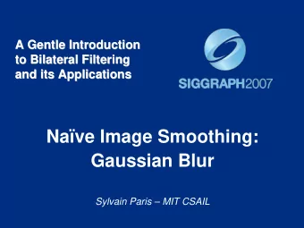
A Gentle Introduction to Bilateral Filtering and its Applications “Fixing the Gaussian Blur”: the Bilateral Filter Sylvain Paris – MIT CSAIL

Blur Comes from Averaging across Edges * output input * * Same Gaussian kernel everywhere.

Properties of Gaussian Blur input • Does smooth images • But smoothes too much: edges are blurred . – Only spatial distance matters output – No edge term      [ ] || || GB I G p q I  p q  q S space

Bilateral Filter [Aurich 95, Smith 97, Tomasi 98] No Averaging across Edges * output input * * The kernel shape depends on the image content.

Bilateral Filter Definition: an Additional Edge Term Same idea: weighted average of pixels . new not new new   1       [ ] || || | | BF I G p q G I I I   p p q q s r W  q S p normalization space weight range weight factor I

Illustration a 1D Image • 1D image = line of pixels • Better visualized as a plot pixel intensity pixel position

Gaussian Blur and Bilateral Filter Gaussian blur p      [ ] || || GB I G p q I  q p q  q S space space Bilateral filter [Aurich 95, Smith 97, Tomasi 98] p range   1       [ ] || || | | p q BF I G G I I I   p p q q W s r  q q S p space range normalization space

Bilateral Filter on a Height Field   1       [ ] || || | | BF I G p q G I I I   p p q q W s r  q S p p p q output input reproduced from [Durand 02]

Space and Range Parameters   1       [ ] || || | | BF I G p q G I I I   p p q q W s r  q S p • space  s : spatial extent of the kernel, size of the considered neighborhood. • range  r : “minimum” amplitude of an edge

Influence of Pixels Only pixels close in space and in range are considered. space range p

Exploring the Parameter Space  r =   r = 0.1  r = 0.25 (Gaussian blur) input  s = 2  s = 6  s = 18

Varying the Range Parameter  r =   r = 0.1  r = 0.25 (Gaussian blur) input  s = 2  s = 6  s = 18

input

 r = 0.1

 r = 0.25

 r =  (Gaussian blur)

Varying the Space Parameter  r =   r = 0.1  r = 0.25 (Gaussian blur) input  s = 2  s = 6  s = 18

input

 s = 2

 s = 6

 s = 18

Basic denoising Noisy input Bilateral filter 7x7 window

Basic denoising Bilateral filter Median 3x3

Basic denoising Bilateral filter Median 5x5

Basic denoising Bilateral filter – lower sigma Bilateral filter

Basic denoising Bilateral filter – higher sigma Bilateral filter