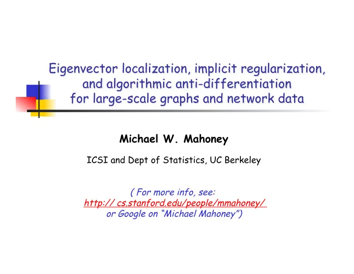
First, parse the title ... Eigenvector localization : Eigenvectors - PowerPoint PPT Presentation

First, parse the title ... Eigenvector localization : • Eigenvectors are “usually” global entities • But they can be localized in extremely sparse/noisy graphs/matrices Implicit regularization: • Usually “exactly” optimize f+ λ g, for some λ and g • Regularization often a side effect of approximations to f Algorithmic anti-differentiation : • What is the objective that approximate computation exactly optimizes Large-scale graphs and network data : • Small versus medium versus large versus big • Social/information networks versus “constructed” graphs

Outline Motivation: large informatics graphs • Downward-sloping, flat, and upward-sloping NCPs (i.e., not “nice” at large size scales , but instead expander-like/tree-like) • Implicit regularization in graph approximation algorithms Eigenvector localization & semi-supervised eigenvectors • Strongly and weakly local diffusions • Extension to semi-supervised eigenvectors Implicit regularization & algorithmic anti-differentiation • Early stopping in iterative diffusion algorithms • Truncation in diffusion algorithms

Outline Motivation: large informatics graphs • Downward-sloping, flat, and upward-sloping NCPs (i.e., not “nice” at large size scales , but instead expander-like/tree-like) • Implicit regularization in graph approximation algorithms Eigenvector localization & semi-supervised eigenvectors • Strongly and weakly local diffusions • Extension to semi-supervised eigenvectors Implicit regularization & algorithmic anti-differentiation • Early stopping in iterative diffusion algorithms • Truncation in diffusion algorithms

Networks and networked data Interaction graph model of Lots of “networked” data!! networks: • technological networks • Nodes represent “entities” – AS, power-grid, road networks • Edges represent “interaction” • biological networks between pairs of entities – food-web, protein networks • social networks – collaboration networks, friendships • information networks – co-citation, blog cross-postings, advertiser-bidded phrase graphs... • language networks – semantic networks... • ...

What do these networks “look” like?

Possible ways a graph might look Low-dimensional structure Core-periphery structure Expander or complete graph Bipartite structure

Scatter plot of λ 2 for real networks Question: does this plot really tell us much about these networks?

Communities, Conductance, and NCPPs Let A be the adjacency matrix of G=(V,E). The conductance φ of a set S of nodes is: The Network Community Profile (NCP) Plot of the graph is: Just as conductance captures a Surface-Area-To-Volume notion • the NCP captures a Size-Resolved Surface-Area-To-Volume notion • captures the idea of size-resolved bottlenecks to diffusion

Why worry about both criteria? • Some graphs (e.g., “space-like” graphs, finite element meshes, road networks, random geometric graphs) cut quality and cut balance “work together” • For other classes of graphs (e.g., informatics graphs, as we will see) there is a “tradeoff,” i.e., better cuts lead to worse balance • For still other graphs (e.g., expanders) there are no good cuts of any size

Probing Large Networks with Approximation Algorithms Idea : Use approximation algorithms for NP-hard graph partitioning problems as experimental probes of network structure. Spectral - (quadratic approx) - confuses “long paths” with “deep cuts” Multi-commodity flow - (log(n) approx) - difficulty with expanders SDP - (sqrt(log(n)) approx) - best in theory Metis - (multi-resolution for mesh-like graphs) - common in practice X+MQI - post-processing step on, e.g., Spectral of Metis Metis+MQI - best conductance (empirically) Local Spectral - connected and tighter sets (empirically, regularized communities!) • We exploit the “statistical” properties implicit in “worst case” algorithms.

Typical intuitive networks Newman’s Network Science Zachary’s karate club d-dimensional meshes RoadNet-CA

Typical real network General relativity collaboration network (4,158 nodes, 13,422 edges) Data are expander-like at large size scales !!! Community ¡score ¡ Community ¡size ¡ 13 ¡

“Whiskers” and the “core” • “Whiskers” • maximal sub-graph detached from network by removing a single edge • contains 40% of nodes and 20% of edges • “Core” • the rest of the graph, i.e., the 2-edge-connected core • Global minimum of NCPP is a whisker NCP ¡plot ¡ • And, the core has a core-peripehery structure, recursively ... Slope ¡upward ¡as ¡cut ¡ Largest ¡ into ¡core ¡ ¡ whisker ¡

A simple theorem on random graphs Structure of the G(w) model, with β ε (2,3). • Sparsity (coupled with randomness) is the issue, not heavy-tails. • (Power laws with β ε (2,3) give us Power-law random graph with β ε (2,3). the appropriate sparsity.) Think of the data as: local-structure on global-noise; not small noise on global structure!

Three different types of real networks NCP: conductance value of best conductance CRP: ratio of internal to external conductance, set in graph, as a function of size as a function of size CA-GrQc FB-Johns55 US-Senate

Local structure for graphs with upward versus downward sloping NCPs CA-GrQc: upward- AclCut (strongly local sloping global NCP spectral method) versus MovCut (weakly local spectral method) Two very similar FB-Johns55: flat methods often give global NCP very different results. Former is often preferable---for both algorithmic and statistical reasons. US-Senate: downward- Why? And what does sloping global NCP problem does it solve?

Regularized and non-regularized communities Diameter of the cluster Conductance of bounding cut Local Spectral Connected Disconnected External/internal conductance Lower is good • Metis+MQI - a Flow-based method (red) gives sets with better conductance. • Local Spectral (blue) gives tighter and more well-rounded sets.

Summary of lessons learned Local-global properties of real data are very different ... • ... than practical/theoretical people implicitly/explicitly assume Local spectral methods were a big winner • For both algorithmic and statistical reasons Little design decisions made a big difference • Details of how deal with truncation and boundary conditions are not second- order issues when graphs are expander-like Approximation algorithm usefulness uncoupled from theory • Often useful when they implicitly regularize

Outline Motivation: large informatics graphs • Downward-sloping, flat, and upward-sloping NCPs (i.e., not “nice” at large size scales , but instead expander-like/tree-like) • Implicit regularization in graph approximation algorithms Eigenvector localization & semi-supervised eigenvectors • Strongly and weakly local diffusions • Extension to semi-supervised eigenvectors Implicit regularization & algorithmic anti-differentiation • Early stopping in iterative diffusion algorithms • Truncation in diffusion algorithms

Local spectral optimization methods Local spectral methods - provably-good local version of global spectral ST04: truncated “local” random walks to compute locally-biased cut ACL06: approximate locally-biased PageRank vector computations Chung08: approximate heat-kernel computation to get a vector Q1: What do these procedures optimize approximately/exactly? Q2: Can we write these procedures as optimization programs?

Recall spectral graph partitioning • Relaxation of: The basic optimization problem: • Solvable via the eigenvalue problem: • Sweep cut of second eigenvector yields: Also recall Mihail’s sweep cut for a general test vector:

Geometric correlation and generalized PageRank vectors Can use this to define a geometric Given a cut T, define the notion of correlation between cuts: vector: • PageRank: a spectral ranking method (regularized version of second eigenvector of L G ) • Personalized: s is nonuniform; & generalized: teleportation parameter α can be negative.

Local spectral partitioning ansatz Mahoney, Orecchia, and Vishnoi (2010) Primal program: Dual program: Interpretation: Interpretation: • Find a cut well-correlated with the • Embedding a combination of scaled seed vector s. complete graph K n and complete graphs T and T (K T and K T ) - where • If s is a single node, this relax: the latter encourage cuts near (T,T).

Main results (1 of 2) Mahoney, Orecchia, and Vishnoi (2010) Theorem : If x* is an optimal solution to LocalSpectral, it is a GPPR vector for parameter α , and it can be computed as the solution to a set of linear equations. Proof: (1) Relax non-convex problem to convex SDP (2) Strong duality holds for this SDP (3) Solution to SDP is rank one (from comp. slack.) (4) Rank one solution is GPPR vector.

Main results (2 of 2) Mahoney, Orecchia, and Vishnoi (2010) Theorem : If x* is optimal solution to LocalSpect (G,s, κ ), one can find a cut of conductance ≤ 8 λ (G,s, κ ) in time O(n lg n) with sweep cut of x*. Upper bound, as usual from sweep cut & Cheeger. Theorem : Let s be seed vector and κ correlation parameter. For all sets of nodes T s.t. κ ’ :=<s,s T > D 2 , we have: φ (T) ≥ λ (G,s, κ ) if κ ≤ κ ’, and φ (T) ≥ ( κ ’/ κ ) λ (G,s, κ ) if κ ’ ≤ κ . Lower bound: Spectral version of flow- improvement algs.