Introduction to Mobile Robotics SLAM: Simultaneous Localization - PowerPoint PPT Presentation
Introduction to Mobile Robotics SLAM: Simultaneous Localization and Mapping Wolfram Burgard, Cyrill Stachniss, Kai Arras, Maren Bennewitz What is SLAM? Estimate the pose of a robot and the map of the environment at the same time
Introduction to Mobile Robotics SLAM: Simultaneous Localization and Mapping Wolfram Burgard, Cyrill Stachniss, Kai Arras, Maren Bennewitz
What is SLAM? § Estimate the pose of a robot and the map of the environment at the same time § SLAM is hard, because § a map is needed for localization and § a good pose estimate is needed for mapping § Localization: inferring location given a map § Mapping: inferring a map given locations § SLAM: learning a map and locating the robot simultaneously
The SLAM Problem § SLAM is a chicken-or-egg problem: → a map is needed for localization and → a pose estimate is needed for mapping 3
SLAM Applications § SLAM is central to a range of indoor, outdoor, in-air and underwater applications for both manned and autonomous vehicles. Examples: § At home: vacuum cleaner, lawn mower § Air: surveillance with unmanned air vehicles § Underwater: reef monitoring § Underground: exploration of mines § Space: terrain mapping for localization 4
SLAM Applications Indoors Undersea Space Underground 5
Map Representations Examples: Subway map, city map, landmark-based map Maps are topological and/or metric models of the environment 6
Map Representations in Robotics § Grid maps or scans, 2d, 3d [Lu & Milios, 97; Gutmann, 98: Thrun 98; Burgard, 99; Konolige & Gutmann, 00; Thrun, 00; Arras, 99; Haehnel, 01; Grisetti et al., 05; …] § Landmark-based [Leonard et al., 98; Castelanos et al., 99: Dissanayake et al., 2001; Montemerlo et al., 2002;… 7
The SLAM Problem § SLAM is considered a fundamental problems for robots to become truly autonomous § Large variety of different SLAM approaches have been developed § The majority uses probabilistic concepts § History of SLAM dates back to the mid-eighties 8
Feature-Based SLAM Given: § The robot ’ s controls § Relative observations Wanted: § Map of features § Path of the robot 9
Feature-Based SLAM § Absolute robot poses § Absolute landmark positions § But only relative measurements of landmarks 10
Why is SLAM a hard problem? 1. Robot path and map are both unknown 2. Errors in map and pose estimates correlated 11
Why is SLAM a hard problem? § The mapping between observations and landmarks is unknown § Picking wrong data associations can have catastrophic consequences (divergence) Robot pose uncertainty 12
SLAM: Simultaneous Localization And Mapping § Full SLAM: p ( x 0: t , m | z 1: t , u 1: t ) Estimates entire path and map! § Online SLAM: … ∫ ∫ ∫ p ( x t , m | z 1: t , u 1: t ) = p ( x 1: t , m | z 1: t , u 1: t ) dx 1 dx 2 ... dx t − 1 Estimates most recent pose and map! § Integrations (marginalization) typically done recursively, one at a time 13
Graphical Model of Full SLAM p ( x , m | z , u ) 1 : t 1 : t 1 : t 14
Graphical Model of Online SLAM p ( x , m | z , u ) … p ( x , m | z , u ) dx dx ... dx = ∫∫ ∫ t 1 : t 1 : t 1 : t 1 : t 1 : t 1 2 t 1 − 15
Motion and Observation Model "Motion model" "Observation model" 16
Remember the KF Algorithm 1. Algorithm Kalman_filter ( µ t-1 , Σ t-1 , u t , z t ): 2. Prediction: 3. A B u µ = µ + t t t − 1 t t 4. T A A R Σ = Σ + t t t − 1 t t 5. Correction: T T 1 6. K C ( C C Q ) − = Σ Σ + t t t t t t t K ( z C ) 7. µ = µ + − µ t t t t t t 8. ( I K C ) Σ = − Σ t t t t 9. Return µ t , Σ t 17
EKF SLAM: State representation § Localization 3x1 pose vector 3x3 cov. matrix § SLAM Landmarks simply extend the state. Growing state vector and covariance matrix! 18
EKF SLAM: State representation § Map with n landmarks: (3+2 n )-dimensional Gaussian # & 2 # & x σ x σ xy σ x θ σ xl 1 σ xl 2 σ xl N % ( % ( 2 y σ xy σ y σ y θ σ yl 1 σ yl 2 σ yl N % ( % ( % ( 2 % ( θ σ x θ σ y θ σ θ σ θ l 1 σ θ l 2 σ θ l N % ( % ( 2 σ l 1 l N Bel ( x t , m t ) = l 1 , σ xl 1 σ yl 1 σ θ l 1 σ l 1 σ l 1 l 2 % ( % ( 2 σ l 2 l N % ( % l 2 ( σ xl 2 σ yl 2 σ θ l 2 σ l 1 l 2 σ l 2 % ( % ( % ( % ( % ( % ( 2 l N σ xl N σ yl N σ θ l N σ l 1 l N σ l 2 l N σ l N $ ' $ ' § Can handle hundreds of dimensions 19
EKF SLAM: Building the Map Filter Cycle , Overview: 1. State prediction (odometry) 2. Measurement prediction 3. Observation 4. Data Association 5. Update 6. Integration of new landmarks 20
EKF SLAM: Building the Map § State Prediction Odometry: Robot-landmark cross- covariance prediction: (skipping time index k ) 21
EKF SLAM: Building the Map § Measurement Prediction Global-to-local frame transform h 22
EKF SLAM: Building the Map § Observation (x,y) -point landmarks 23
EKF SLAM: Building the Map § Data Association Associates predicted measurements with observation ? 24
EKF SLAM: Building the Map § Filter Update The usual Kalman filter expressions 25
EKF SLAM: Building the Map § Integrating New Landmarks State augmented by Cross-covariances: 26
EKF SLAM Map Correlation matrix 27
EKF SLAM Map Correlation matrix 28
EKF SLAM Map Correlation matrix 29
EKF SLAM: Correlations Matter § What if we neglected cross-correlations? 30
EKF SLAM: Correlations Matter § What if we neglected cross-correlations? § Landmark and robot uncertainties would become overly optimistic § Data association would fail § Multiple map entries of the same landmark § Inconsistent map 31
SLAM: Loop Closure § Recognizing an already mapped area , typically after a long exploration path (the robot "closes a loop”) § Structurally identical to data association, but § high levels of ambiguity § possibly useless validation gates § environment symmetries § Uncertainties collapse after a loop closure (whether the closure was correct or not) 36
SLAM: Loop Closure § Before loop closure 37
SLAM: Loop Closure § After loop closure 38
SLAM: Loop Closure § By revisiting already mapped areas, uncertainties in robot and landmark estimates can be reduced § This can be exploited when exploring an environment for the sake of better (e.g. more accurate) maps § Exploration: the problem of where to acquire new information → See separate chapter on exploration 39
KF-SLAM Properties (Linear Case) § The determinant of any sub-matrix of the map covariance matrix decreases monotonically as successive observations are made § When a new land- mark is initialized, its uncertainty is maximal § Landmark uncer- tainty decreases monotonically with each new observation [Dissanayake et al., 2001] 40
KF-SLAM Properties (Linear Case) § In the limit, the landmark estimates become fully correlated [Dissanayake et al., 2001] 41
KF-SLAM Properties (Linear Case) § In the limit, the covariance associated with any single landmark location estimate is determined only by the initial covariance in the vehicle location estimate . [Dissanayake et al., 2001] 42
EKF SLAM Example: Victoria Park Dataset 43
Victoria Park: Data Acquisition [courtesy by E. Nebot] 44
Victoria Park: Estimated Trajectory [courtesy by E. Nebot] 45
Victoria Park: Landmarks [courtesy by E. Nebot] 46
EKF SLAM Example: Tennis Court [courtesy by J. Leonard] 47
EKF SLAM Example: Tennis Court odometry estimated trajectory [courtesy by John Leonard] 48
EKF SLAM Example: Line Features § KTH Bakery Data Set [Wulf et al., ICRA 04] 49
EKF-SLAM: Complexity § Cost per step: quadratic in n, the number of landmarks: O(n 2 ) § Total cost to build a map with n landmarks: O(n 3 ) § Memory consumption: O(n 2 ) § Problem: becomes computationally intractable for large maps! § There exists variants to circumvent these problems 50
SLAM Techniques § EKF SLAM § FastSLAM § Graph-based SLAM § Topological SLAM (mainly place recognition) § Scan Matching / Visual Odometry (only locally consistent maps) § Approximations for SLAM: Local submaps, Sparse extended information filters, Sparse links, Thin junction tree filters, etc. § … 51
EKF-SLAM: Summary § The first SLAM solution § Convergence proof for linear Gaussian case § Can diverge if nonlinearities are large (and the reality is nonlinear...) § Can deal only with a single mode § Successful in medium-scale scenes § Approximations exists to reduce the computational complexity 52
Recommend


More recommend
Explore More Topics
Stay informed with curated content and fresh updates.