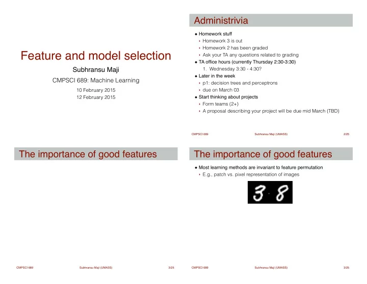

Administrivia Homework stuff ! ‣ Homework 3 is out ‣ Homework 2 has been graded Feature and model selection ‣ Ask your TA any questions related to grading TA office hours (currently Thursday 2:30-3:30) ! Subhransu Maji 1. Wednesday 3:30 - 4:30? Later in the week ! CMPSCI 689: Machine Learning ‣ p1: decision trees and perceptrons ‣ due on March 03 10 February 2015 Start thinking about projects ! 12 February 2015 ‣ Form teams (2+) ‣ A proposal describing your project will be due mid March (TBD) CMPSCI 689 Subhransu Maji (UMASS) 2 /25 The importance of good features The importance of good features Most learning methods are invariant to feature permutation ! ‣ E.g., patch vs. pixel representation of images CMPSCI 689 Subhransu Maji (UMASS) 3 /25 CMPSCI 689 Subhransu Maji (UMASS) 3 /25
The importance of good features The importance of good features Most learning methods are invariant to feature permutation ! Most learning methods are invariant to feature permutation ! ‣ E.g., patch vs. pixel representation of images ‣ E.g., patch vs. pixel representation of images permute pixels permute pixels permute patches bag of pixels bag of pixels bag of patches can you recognize the digits? can you recognize the digits? CMPSCI 689 Subhransu Maji (UMASS) 3 /25 CMPSCI 689 Subhransu Maji (UMASS) 3 /25 Irrelevant and redundant features Irrelevant and redundant features How do irrelevant features affect decision tree classifiers? Irrelevant features ! E [ f ; C ] = E [ f ] ‣ E.g., a binary feature with Consider adding 1 binary noisy feature for a binary classification task ! Redundant features ! ‣ For simplicity assume that in our dataset there are N/2 instances ‣ For example, pixels next to each other are highly correlated label=+1 and N/2 instances with label=-1 Irrelevant features are not that unusual ! ‣ Probability that a noisy feature is perfectly correlated with the labels in the dataset is 2x0.5 ᴺ ‣ Consider bag-of-words model for text which typically have on the order of 100,000 features, but only a handful of them are useful for ‣ Very small if N is large (1e-6 for N=21) spam classification ‣ But things are considerably worse where there are many irrelevant ! features, or if we allow partial correlation ! For large datasets, the decision tree learner can learn to ignore noisy features that are not correlated with the labels. ! Different learning algorithms are affected differently by irrelevant and redundant features CMPSCI 689 Subhransu Maji (UMASS) 4 /25 CMPSCI 689 Subhransu Maji (UMASS) 5 /25
Irrelevant and redundant features Irrelevant and redundant features How do irrelevant features affect kNN classifiers? How do irrelevant features affect perceptron classifiers? Perceptrons can learn low weight on irrelevant features ! kNN classifiers (with Euclidean distance) treat all the features equally ! Irrelevant features can affect the convergence rate ! Noisy dimensions can dominate distance computation ! ‣ updates are wasted on learning low weights on irrelevant features Randomly distributed points in high dimensions are all (roughly) equally apart! ! But like decision trees, if the dataset is large enough, the perceptron will eventually learn to ignore the weights ! ! Effect of noise on classifiers: ! a i ← N (0 , 1) b i ← N (0 , 1) ! “3” vs “8” classification using pixel features ! √ (28x28 images = 784 features) E [ || a − b || ] → 2 D ! ! ! ! i = 2 0 , . . . , 2 12 x ← [ x z ] z i = N (0 , 1) , kNN classifiers can be bad with noisy features even for large N vary the number of noisy dimensions CMPSCI 689 Subhransu Maji (UMASS) 6 /25 CMPSCI 689 Subhransu Maji (UMASS) 7 /25 Feature selection Feature selection methods Selecting a small subset of useful features ! Reasons: ! ‣ Reduce measurement cost ‣ Reduces data set and resulting model size ‣ Some algorithms scale poorly with increased dimension ‣ Irrelevant features can confuse some algorithms ‣ Redundant features adversely affect generalization for some learning methods ‣ Removal of features can make learning easier and improve generalization (for example by increasing the margin) CMPSCI 689 Subhransu Maji (UMASS) 8 /25 CMPSCI 689 Subhransu Maji (UMASS) 9 /25
Feature selection methods Feature selection methods Methods agnostic to the learning algorithm Methods agnostic to the learning algorithm ‣ Surface heuristics: remove a feature if it rarely changes CMPSCI 689 Subhransu Maji (UMASS) 9 /25 CMPSCI 689 Subhransu Maji (UMASS) 9 /25 Feature selection methods Feature selection methods Methods agnostic to the learning algorithm Methods agnostic to the learning algorithm ‣ Surface heuristics: remove a feature if it rarely changes ‣ Surface heuristics: remove a feature if it rarely changes ‣ Ranking based: rank features according to some criteria ‣ Ranking based: rank features according to some criteria ➡ Correlation: scatter plot CMPSCI 689 Subhransu Maji (UMASS) 9 /25 CMPSCI 689 Subhransu Maji (UMASS) 9 /25
Feature selection methods Feature selection methods Methods agnostic to the learning algorithm Methods agnostic to the learning algorithm ‣ Surface heuristics: remove a feature if it rarely changes ‣ Surface heuristics: remove a feature if it rarely changes ‣ Ranking based: rank features according to some criteria ‣ Ranking based: rank features according to some criteria ➡ Correlation: ➡ Correlation: scatter plot scatter plot ➡ Mutual information: ➡ Mutual information: X entropy X entropy H ( X ) = − p ( x ) log p ( x ) H ( X ) = − p ( x ) log p ( x ) x x decision ! decision ! trees? trees? ‣ Usually cheap CMPSCI 689 Subhransu Maji (UMASS) 9 /25 CMPSCI 689 Subhransu Maji (UMASS) 9 /25 Feature selection methods Forward and backward selection Methods agnostic to the learning algorithm ‣ Surface heuristics: remove a feature if it rarely changes ‣ Ranking based: rank features according to some criteria ➡ Correlation: scatter plot ➡ Mutual information: X entropy H ( X ) = − p ( x ) log p ( x ) x decision ! trees? ‣ Usually cheap Wrapper methods ‣ Aware of the learning algorithm (forward and backward selection) ‣ Can be computationally expensive CMPSCI 689 Subhransu Maji (UMASS) 9 /25 CMPSCI 689 Subhransu Maji (UMASS) 10 /25
Forward and backward selection Forward and backward selection Given: a learner L, a dictionary of features D to select from Given: a learner L, a dictionary of features D to select from ‣ E.g., L = kNN classifier, D = polynomial functions of features ‣ E.g., L = kNN classifier, D = polynomial functions of features Forward selection ! Forward selection ! ‣ Start with an empty set of features F = Φ ‣ Start with an empty set of features F = Φ ‣ Repeat till |F| < n ‣ Repeat till |F| < n ➡ For every f in D ➡ For every f in D • Evaluate the performance of the learner on F ∪ f • Evaluate the performance of the learner on F ∪ f ➡ Pick the best feature f* ➡ Pick the best feature f* ➡ F = F ∪ f*, D = D \ f* ➡ F = F ∪ f*, D = D \ f* Backward selection is similar ! ‣ Initialize F = D, and iteratively remove the feature that is least useful ‣ Much slower than forward selection CMPSCI 689 Subhransu Maji (UMASS) 10 /25 CMPSCI 689 Subhransu Maji (UMASS) 10 /25 Forward and backward selection Approximate feature selection Given: a learner L, a dictionary of features D to select from What if the number of potential features are very large? ! ‣ E.g., L = kNN classifier, D = polynomial functions of features ‣ If may be hard to find the optimal feature Forward selection ! ! ‣ Start with an empty set of features F = Φ ! ‣ Repeat till |F| < n ! ➡ For every f in D ! • Evaluate the performance of the learner on F ∪ f [Viola and Jones, IJCV 01] ! ➡ Pick the best feature f* ! ➡ F = F ∪ f*, D = D \ f* ! Backward selection is similar ! ! Approximation by sampling: pick the best among a random subset ! ‣ Initialize F = D, and iteratively remove the feature that is least useful If done during decision tree learning, this will give you a random tree ! ‣ Much slower than forward selection ‣ We will see later (in the lecture on ensemble learning ) that it is good Greedy, but can be near optimal under certain conditions to train many random trees and average them (random forest). CMPSCI 689 Subhransu Maji (UMASS) 10 /25 CMPSCI 689 Subhransu Maji (UMASS) 11 /25
Feature normalization Feature normalization Even if a feature is useful some normalization may be good CMPSCI 689 Subhransu Maji (UMASS) 12 /25 CMPSCI 689 Subhransu Maji (UMASS) 12 /25 Feature normalization Feature normalization Even if a feature is useful some normalization may be good Even if a feature is useful some normalization may be good Per-feature normalization Per-feature normalization µ d = 1 µ d = 1 X X ‣ Centering x n,d ‣ Centering x n,d x n,d ← x n,d − µ d x n,d ← x n,d − µ d N N n n s s 1 1 x n,d ← x n,d / σ d x n,d ← x n,d / σ d ‣ Variance scaling X ‣ Variance scaling X σ d = ( x n,d − µ d ) 2 σ d = ( x n,d − µ d ) 2 N N n n ‣ Absolute scaling x n,d ← x n,d /r d ‣ Absolute scaling x n,d ← x n,d /r d | x n,d | | x n,d | r d = max r d = max n n ‣ Non-linear transformation Caltech-101 image classification ➡ square-root x n,d ← √ x n,d 41.6% linear ! 63.8% square-root (corrects for burstiness) CMPSCI 689 Subhransu Maji (UMASS) 12 /25 CMPSCI 689 Subhransu Maji (UMASS) 12 /25
Recommend
More recommend