A Bayesian method to detect targets of selection in - PowerPoint PPT Presentation
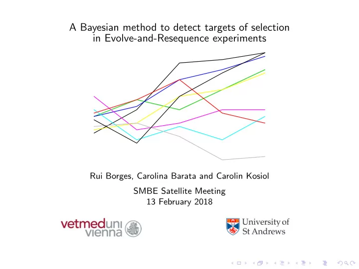
A Bayesian method to detect targets of selection in Evolve-and-Resequence experiments Rui Borges, Carolina Barata and Carolin Kosiol SMBE Satellite Meeting 13 February 2018 Natural selection Natural selection is a key force in evolution
A Bayesian method to detect targets of selection in Evolve-and-Resequence experiments Rui Borges, Carolina Barata and Carolin Kosiol SMBE Satellite Meeting 13 February 2018
Natural selection ◮ Natural selection is a key force in evolution ◮ Mechanisms by which populations can adapt to external pressures ◮ We focus on the adaptive evolution due to standing variation in fixed-size populations
Selection and experimental evolution Replicates Pressure Evolve . . . Cage Sequencing Time t0 Time t1 Time tN ◮ Evolve-and-Resequence experiments: pool-seq time series data
Testing/measuring adaptive scenarios Mechanistic methods Empirical methods ◮ WFABC ◮ Fisher exact test (Foll et al. 2015) ◮ CMH test ◮ Clear (Agresti and Kateri 2011) (Iranmehr et al. 2017) ◮ Gaussian processes ◮ LLS (Topa et al. 2015) (Taus et al. 20157)
Measuring adaptive scenarios WFABC Clear LLS ◮ LRTs ◮ Least squares ◮ Bayes factors ◮ Empirical p-values ◮ Empirical p-values ◮ Highly dependent based on based on on the summary genome-wide drift simulations of allele statistics simulations trajectories
Improvements to existing methods ◮ Full picture: distribution of σ ◮ Computationally fast, allowing genome-wide applications
Defining population states ◮ Consider two alleles A and a and a population of fixed size N ◮ Population states: { nA , ( N − n ) a } { 2 A , 8 a }
Evolving population states {1A,9a} {3A,7a} {7A,3a} ◮ Trajectory X t is a collection of states { nA , ( N − n ) a } informing the number of alleles A on time t ◮ According to the Moran model with selection (Moran 1958) n ( N − n ) n → n − 1 : N n ( N − n ) n → n + 1 : (1 + σ ) N ◮ Neutrality: σ = 0
The likelihood function ◮ X t : number of alleles A on time t ◮ T : number of time points ◮ R : number or replicates R T � p ( X r 0 = x r � p ( X r t = x r t | X r t − 1 = x r p ( X | σ ) = 0 ) t − 1 , σ ) r =1 t =1
Sequencing noise ◮ allele counts indirectly inform on the frequency of an allele in a population ◮ binomial sampling process � � � n C � c � 1 − n � C − c p ( { nA , ( N − n ) a } | c ) ∝ c N N
Algorithm ◮ Calculates the allele trajectories ◮ Calculates the likelihood/posterior given σ ◮ Adjusts the the log posterior using orthogonal polynomials ◮ Calculates summary statistics: ˆ σ and BF sync fi le log posterior allele trajectories
Algorithm: example N e σ = 10 C = 40 x BF = 5 . 7 CPU time = 1 second Burke et al. (2014) dataset (75500 sites) = 21 hours
Simulated data Experimental conditions : Population scenarios : ◮ Number of replicates ◮ Effective population size ◮ Time schemes ◮ Strength of selection ◮ Coverage ◮ Allele initial frequency
Number of replicates ◮ Higher number of replicates lead to unbiased and narrower ˆ σ ◮ Two replicates are likely to lead to erroneous conclusions, specially in regimens of selection Genetic drift < Selection Ne=300 Ne σ =10 15 scaled selection coe ffi cient 10 5 0 -5 5 10 2 Replicates Initial frequency: 0.01 0.05 0.1 0.5 true σ
Time schemes Genetic drift < Selection Genetic drift < Selection Ne=300 Ne σ =10 Tmax=Ne/4 Ne=300 Ne σ =10 Tmax=Ne/2 scaled selection coe ffi cient 15 15 10 10 5 5 0 -5 0 -10 -5 2 5 10 2 5 10 Number of time points Number of time points Initial frequency: 0.01 0.05 0.1 0.5 true σ Time schemes: uniform more sampling at the begginig more sampling at the end ◮ ˆ σ are less biased for more time points ◮ more sampling at the begging improves ˆ σ , specially in regimens of selection ◮ Two time points are likely to lead to erroneous conclusions
Coverage ◮ Coverage does not seem to significantly interfere with ˆ σ Genetic drift < Selection Ne=300 Ne σ =10 scaled selection coe ffi cient 15 10 5 0 -5 -10 20x 60x 100x 200x Coverage Initial frequency: 0.01 0.05 0.1 0.5 true σ
Our method vs. LLS 0.03 0.2 0.01 σ LLS σ LLS 0.1 ^ ^ -0.01 0.0 Ne=300 Ne=300 Ne σ =1 Ne σ =1 -0.1 -0.03 p0=0.01 p0=0.5 -0.1 0.0 0.1 0.2 -0.03 -0.01 0.01 0.03 ^ ^ σ our algorithm σ our algorithm bias of σ with LLS ^ ^ bias of σ with our algorithm true σ ◮ LLS overestimates σ for trajectories starting with lower frequencies ◮ both methods perform quite similar for trajectories starting with higher frequencies
Application to real data Drosophila simulans dataset (Barghi et al. 2019) ◮ 10 replicates ◮ sequencing at 7 time points: 0, 10, ..., 60 ◮ N e ≈ 300 Chromosome X selective SNPs 10 neutral SNPs 8 |log BF| 6 4 2 0 0.0e+00 5.0e+06 1.0e+07 1.5e+07 2.0e+07 Genomic position
Application to real data Chromosome 3R 0.00012 neutral SNPs selective SNPs 0.00008 variance σ 0.00004 0.00000 -0.03 -0.02 -0.01 0.00 0.01 0.02 average σ ◮ variance of σ measures the heterogeneity of allele trajectories among replicates ◮ identify SNP with different adaptive strategies
Summary and future work ◮ Distribution of σ ◮ Statistically cleaner ◮ Computationally fast ◮ Flexible tool ◮ More testing in real datasets (suggestions?) ◮ Multiple testing scheme for the BFs
Acknowledgements ◮ Claus Vogel ◮ Neda Barghi ◮ Marta Pelizzola ◮ WWTF Project MA16-061 Centre for Biological Diversity Institute of Population Genetics University of St Andrews Vetmeduni Vienna
Recommend
More recommend
Explore More Topics
Stay informed with curated content and fresh updates.
