Fast Regularization Paths via Coordinate Descent Trevor Hastie - PowerPoint PPT Presentation

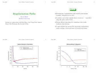
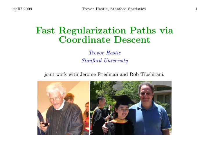
useR! 2009 Trevor Hastie, Stanford Statistics 1 Fast Regularization Paths via Coordinate Descent Trevor Hastie Stanford University joint work with Jerome Friedman and Rob Tibshirani.

useR! 2009 Trevor Hastie, Stanford Statistics 2 Linear Models in Data Mining As datasets grow wide —i.e. many more features than samples—the linear model has regained favor in the dataminers toolbox. Document classification: bag-of-words can leads to p = 20 K features and N = 5 K document samples. Image deblurring, classification: p = 65 K pixels are features, N = 100 samples. Genomics, microarray studies: p = 40 K genes are measured for each of N = 100 subjects. Genome-wide association studies: p = 500 K SNPs measured for N = 2000 case-control subjects. In all of these we use linear models — e.g. linear regression, logistic regression. Since p ≫ N , we have to regularize.

useR! 2009 Trevor Hastie, Stanford Statistics 3 February 2009. Additional chapters on wide data, random forests, graphical models and ensemble methods + new material on path algorithms, kernel methods and more.

useR! 2009 Trevor Hastie, Stanford Statistics 4 Linear regression via the Lasso (Tibshirani, 1995) • Given observations { y i , x i 1 , . . . , x ip } N i =1 p p N x ij β j ) 2 subject to � � � min ( y i − β 0 − | β j | ≤ t β i =1 j =1 j =1 j β 2 • Similar to ridge regression , which has constraint � j ≤ t • Lasso does variable selection and shrinkage, while ridge only shrinks. . . β 2 β ^ ^ 2 β β β 1 β 1

useR! 2009 Trevor Hastie, Stanford Statistics 5 Brief History of ℓ 1 Regularization • Wavelet Soft Thresholding (Donoho and Johnstone 1994) in orthonormal setting. • Tibshirani introduces Lasso for regression in 1995. • Same idea used in Basis Pursuit (Chen, Donoho and Saunders 1996). • Extended to many linear-model settings e.g. Survival models (Tibshirani, 1997), logistic regression, and so on. • Gives rise to a new field Compressed Sensing (Donoho 2004, Candes and Tao 2005)—near exact recovery of sparse signals in very high dimensions. In many cases ℓ 1 a good surrogate for ℓ 0 .

useR! 2009 Trevor Hastie, Stanford Statistics 6 Lasso Coefficient Path 0 2 3 4 5 7 8 10 9 Standardized Coefficients 500 6 4 8 10 0 1 2 − 500 5 0.0 0.2 0.4 0.6 0.8 1.0 || ˆ β ( λ ) || 1 / || ˆ β (0) || 1 i β ) 2 + λ || β || 1 Lasso: ˆ � N i =1 ( y i − β 0 − x T β ( λ ) = argmin β

useR! 2009 Trevor Hastie, Stanford Statistics 7 History of Path Algorithms Efficient path algorithms for ˆ β ( λ ) allow for easy and exact cross-validation and model selection. • In 2001 the LARS algorithm (Efron et al) provides a way to compute the entire lasso coefficient path efficiently at the cost of a full least-squares fit. • 2001 – present: path algorithms pop up for a wide variety of related problems: Grouped lasso (Yuan & Lin 2006), support-vector machine (Hastie, Rosset, Tibshirani & Zhu 2004), elastic net (Zou & Hastie 2004), quantile regression (Li & Zhu, 2007), logistic regression and glms (Park & Hastie, 2007), Dantzig selector (James & Radchenko 2008), ... • Many of these do not enjoy the piecewise-linearity of LARS, and seize up on very large problems.

useR! 2009 Trevor Hastie, Stanford Statistics 8 Coordinate Descent • Solve the lasso problem by coordinate descent: optimize each parameter separately, holding all the others fixed. Updates are trivial. Cycle around till coefficients stabilize. • Do this on a grid of λ values, from λ max down to λ min (uniform on log scale), using warms starts. • Can do this with a variety of loss functions and additive penalties. Coordinate descent achieves dramatic speedups over all competitors, by factors of 10, 100 and more.

useR! 2009 Trevor Hastie, Stanford Statistics 9 LARS and GLMNET 20 Coefficients 0 − 20 − 40 0 50 100 150 L1 Norm

useR! 2009 Trevor Hastie, Stanford Statistics 10 Speed Trials Competitors: lars As implemented in R package, for squared-error loss. glmnet Fortran based R package using coordinate descent — topic of this talk. Does squared error and logistic (2- and K -class). l1logreg Lasso-logistic regression package by Koh, Kim and Boyd, using state-of-art interior point methods for convex optimization. BBR/BMR Bayesian binomial/multinomial regression package by Genkin, Lewis and Madigan. Also uses coordinate descent to compute posterior mode with Laplace prior—the lasso fit. Based on simulations (next 3 slides) and real data (4th slide).

useR! 2009 Trevor Hastie, Stanford Statistics 11 Linear Regression — Dense Features Average Correlation between Features 0 0.1 0.2 0.5 0.9 0.95 N = 5000 , p = 100 0.05 0.05 0.05 0.05 0.05 0.05 glmnet 0.29 0.29 0.29 0.30 0.29 0.29 lars N = 100 , p = 50000 2.66 2.46 2.84 3.53 3.39 2.43 glmnet 58.68 64.00 64.79 58.20 66.39 79.79 lars Timings (secs) for glmnet and lars algorithms for linear regression with lasso penalty. Total time for 100 λ values, averaged over 3 runs.

useR! 2009 Trevor Hastie, Stanford Statistics 12 Logistic Regression — Dense Features Average Correlation between Features 0 0.1 0.2 0.5 0.9 0.95 N = 5000 , p = 100 7.89 8.48 9.01 13.39 26.68 26.36 glmnet 239.88 232.00 229.62 229.49 223.19 223.09 l1lognet N = 100 , p = 5000 5.24 4.43 5.12 7.05 7.87 6.05 glmnet 165.02 161.90 163.25 166.50 151.91 135.28 l1lognet Timings (seconds) for logistic models with lasso penalty. Total time for tenfold cross-validation over a grid of 100 λ values.

useR! 2009 Trevor Hastie, Stanford Statistics 13 Logistic Regression — Sparse Features 0 0.1 0.2 0.5 0.9 0.95 N = 10 , 000 , p = 100 3.21 3.02 2.95 3.25 4.58 5.08 glmnet 11.80 11.64 11.58 13.30 12.46 11.83 BBR 45.87 46.63 44.33 43.99 45.60 43.16 l1lognet N = 100 , p = 10 , 000 10.18 10.35 9.93 10.04 9.02 8.91 glmnet 45.72 47.50 47.46 48.49 56.29 60.21 BBR 130.27 124.88 124.18 129.84 137.21 159.54 l1lognet Timings (seconds) for logistic model with lasso penalty and sparse features (95% zeros in X ). Total time for ten-fold cross-validation over a grid of 100 λ values.

useR! 2009 Trevor Hastie, Stanford Statistics 14 Logistic Regression — Real Datasets Name Type N p glmnet l1logreg BBR BMR Dense Cancer 14 class 144 16,063 2.5 mins NA 2.1 hrs Leukemia 2 class 72 3571 2.50 55.0 450 Sparse Internet ad 2 class 2359 1430 5.0 20.9 34.7 Newsgroup 2 class 11,314 777,811 2 mins 3.5 hrs Timings in seconds (unless stated otherwise). For Cancer, Leukemia and Internet-Ad, times are for ten-fold cross-validation over 100 λ values; for Newsgroup we performed a single run with 100 values of λ , with λ min = 0 . 05 λ max .

useR! 2009 Trevor Hastie, Stanford Statistics 15 A brief history of coordinate descent for the lasso 1997 Tibshirani’s student Wenjiang Fu at U. Toronto develops the “shooting algorithm” for the lasso. Tibshirani doesn’t fully appreciate it. .

useR! 2009 Trevor Hastie, Stanford Statistics 16 A brief history of coordinate descent for the lasso 1997 Tibshirani’s student Wenjiang Fu at U. Toronto develops the “shooting algorithm” for the lasso. Tibshirani doesn’t fully appreciate it. 2002 Ingrid Daubechies gives a talk at Stanford, describes a one-at-a-time algorithm for the lasso. Hastie implements it, makes an error, and Hastie +Tibshirani conclude that the method doesn’t work. .

useR! 2009 Trevor Hastie, Stanford Statistics 17 A brief history of coordinate descent for the lasso 1997 Tibshirani’s student Wenjiang Fu at U. Toronto develops the “shooting algorithm” for the lasso. Tibshirani doesn’t fully appreciate it. 2002 Ingrid Daubechies gives a talk at Stanford, describes a one-at-a-time algorithm for the lasso. Hastie implements it, makes an error, and Hastie +Tibshirani conclude that the method doesn’t work. 2006 Friedman is external examiner at PhD oral of Anita van der Kooij (Leiden) who uses coordinate descent for elastic net. Friedman, Hastie + Tibshirani revisit this problem. Others have too — Shevade and Keerthi (2003), Krishnapuram and Hartemink (2005), Genkin, Lewis and Madigan (2007), Wu and Lange (2008), Meier, van de Geer and Buehlmann (2008).

useR! 2009 Trevor Hastie, Stanford Statistics 18 Coordinate descent for the lasso j =1 x ij β j ) 2 + λ � p � N i =1 ( y i − � p 1 min β j =1 | β j | 2 N Suppose the p predictors and response are standardized to have mean zero and variance 1. Initialize all the β j = 0. Cycle over j = 1 , 2 , . . . , p, 1 , 2 , . . . till convergence: • Compute the partial residuals r ij = y i − � k � = j x ik β k . • Compute the simple least squares coefficient of these residuals � N j = 1 on j th predictor: β ∗ i =1 x ij r ij N • Update β j by soft-thresholding : λ (0,0) S ( β ∗ ← j , λ ) β j sign( β ∗ j )( | β ∗ = j | − λ ) +