Fast Anisotropic Smoothing of Multi-Valued Images using - PowerPoint PPT Presentation

Fast Anisotropic Smoothing of Multi-Valued Images using Curvature-Preserving PDE’s David Tschumperlé CNRS UMR 6072 (GREYC/ENSICAEN) - Image Team MIA’2006, Paris/France, Sept. 2006

Presentation Layout • Diffusion PDE’s for Multi-Valued Images : A Quick Review • Introducing Curvature-Preserving PDE’s for Image Regularization • Connections with Line Integral Convolutions and Implementation • Application Results

Presentation Layout ⇒ Diffusion PDE’s for Multi-Valued Images : A Quick Review • Introducing Curvature-Preserving PDE’s for Image Regularization • Connections with Line Integral Convolutions and Implementation • Application Results

PDE’s and Image Regularization • Convolution and Linear PDE (Koenderink[84], Alvarez-Guichard-etal[92], ...) : 4 πt e − x 2+ y 2 1 ∂I I ( t ) = I ( t =0) ∗ G σ ⇐ ⇒ ∂t = ∆ I = div ( ∇ I ) where G σ = 4 t • Nonlinear PDE (Perona-Malik[90], Alvarez [92], ...) : ∂I ∂t = div ( c ( �∇ I � ) ∇ I ) with c : R − → R Noisy image Heat flow Perona-Malik

Regularization PDE’s and Multi-Valued Images • Image I : Ω → N of multi-valued points : vectors ( N = R n ), matrices ( N = M n ). (Alvarez, Aubert, Barlaud, Blanc-Feraud, Blomgren , Charbonnier, Chan , Cohen, Deriche , Kornprobst, Kimmel , Malladi , Munford, Morel, Nordström, Osher, Perona, Malik, Rudin, Sapiro , Sochen , Tschumperlé , Weickert ,...) Color image ( N = R 3 ) Scalar PDE applied on each channel Multi-valued PDE Color image Direction field Tensor field

Basic Regularization Principle • PDE regularization is mainly based on local image smoothing. • Local smoothing rules : – On a edge, smoothing performed only along the edge direction (anisotropic smoothing) . – On homogeneous regions, smoothing performed equally in all directions (isotropic smoothing) . • Generalization : Separating the definition of a smoothing geometry, and the smoothing process itself.

Definition of a smoothing geometry • I : Ω → R n , a multi-valued image. • Computing the local geometry of I , described by the smoothed structure tensor field G σ : �� � ∇ I i ∇ I T ∗ G σ G σ ( x,y ) = i i • Eigenvalues λ + , λ − and Eigenvectors θ + , θ − of G σ are very efficient descriptors of the local configuration of I at ( x, y ) . ⇒ The smoothing is then modelized by a tensor field T from G :  1 f 1 ( s ) = 1+ s p   T = f 1 ( λ + + λ − ) θ − θ T − + f 2 ( λ + + λ − ) θ + θ T with + 1  f 2 ( s ) =  1+ s q

Tensor field representation Top of the Lena hat Corresponding diffusion tensor field T ⇒ Tensor field T tells about the desired smoothing directions and smoothing amplitudes.

How the smoothing is then achieved ? • The smoothing itself is performed by the application of one or several iterations of one of these generic PDE’s : ∂I i ∂I i ∂t = div ( T ∇ I i ) ∂t = trace ( TH i ) or ⇒ Most of existing regularization PDE’s conform with these equations. ⇒ Ideally, such PDE’s comply with the diffusion tensor field T : Tensor-directed PDE applied on a color image.

Issues encountered with above formulations • Slow iterative processes : Several iterations are needed to get a result that is regularized enough (since dt → 0 ). • Problems with Divergence formulations : – Non-unicity of the tensor field : ∃ D 1 � = D 2 , div ( D 1 ∇ I ) = div ( D 2 ∇ I ) . – Tensor shapes not always representative of the intuitive smoothing behavior : D 2 = ∇ I ∇ I T ∂I ⇒ D 1 = Id and ∂t = ∆ I. �∇ I � 2

Issues encountered with above formulations • Problems with Trace formulations : – Better respect of the considered tensor-valued geometry. – But tends to over-smooth high-curvature structures (corners).

Issues encountered with above formulations • Can be understood from the mono-directional smoothing case : ∂I ∂t = Trace ( ww T H ) • Geometrical interpretation in terms of local smoothing by gaussian kernels oriented by w ( x,y ) . 100 200 300 400 500 600 700 800 100 200 300 400 500 600 700 800 • Ideally, we would be able to locally smooth with a kernel that curves itself regarding to the local image structure.

Coming Next... ⇒ Need for specific PDE’s avoiding smoothing of structures having high curvatures.

Presentation Layout • Diffusion PDE’s for Multi-Valued Images : A Quick Review ⇒ Introducing Curvature-Preserving PDE’s for Image Regularization • Connections with Line Integral Convolutions and Implementation • Application Results

Curvature-preserving PDE’s • For the mono-directional case, we propose the following PDE : ∂I i ww T H i + ∇ I T � � ∂t = trace i J w w  ∂ 2 I i ∂ 2 I i   ∂u ∂u  ∂x 2 ∂x ∂y ∂x∂y   where J w = and H i =  .        ∂ 2 I i ∂ 2 I i ∂v ∂v ∂x ∂y ∂y 2 ∂x∂y ⇒ Classical “Trace” formulation + Constraint term depending on the variations of w .

How did the constraint term appear ? • If C X stands for the integral curve of w starting from X = ( x, y ) , and parameterized by a s.a : ∂ C X ( a ) C X = w ( C X (0) = X et ( a ) ) , then : ∂a ∂ 2 C X ∂ C X + h 2 + O ( h 3 ) = X + h w ( X ) + h 2 ( a ) ( a ) 2 J w ( X ) w ( X ) + O ( h 3 ) C X C X = (0) + h ( h ) ∂a 2 2 ∂a | a =0 | a =0 with h → 0 , and O ( h n ) = h n ǫ n . Thus, we get : ! X + h w ( X ) + h 2 2 J w ( X ) w ( X ) + O ( h 3 ) I i ( C X ( h ) ) = I i 2 J w ( X ) w ( X ) ) + h 2 ( X ) ( w ( X ) + h “ ” + O ( h 3 ) T w ( X ) w T = I i ( X ) + h ∇ I i 2 trace ( X ) H i ( X ) • and then... ∂ 2 I i ( C X ( a ) ) 1 h i I i ( C X ( h ) ) + I i ( C X ( − h ) ) − 2 I i ( C X = lim (0) ) ∂a 2 h 2 h → 0 | a =0 1 h 2 ∇ I T i J w ( X ) w ( X ) + h 2 trace h “ ” i w ( X ) w T + O ( h 3 ) = lim ( X ) H i ( X ) h 2 h → 0 “ ” w ( X ) w T + ∇ I T = trace ( X ) H i ( X ) i J w ( X ) w ( X )

Interpretation of the constraint term • Our curvature-preserving PDE can be written as : ∂ 2 I i ( C X ( a ) ) ∂I i | a =0 = ∆ X ∂t = C I i ∂a 2 where C X is the integral line of w starting from X , and parameterized as : ∂ C X ( a ) C X = w ( C X (0) = X and ( a ) ) ∂a • PDE equivalent to a heat flow on the integral lines of w . • If w is chosen to be the directions of the image contours (eigenvector θ − of G σ ), the smoothing will respect the shape of the contour, whatever its curvature is.

Smoothing along integral lines (a) An integral line C X (b) Some integral lines around a triple-junction. ⇒ The performed smoothing will preserve the curved structure.

Extension to a tensor-based geometry • More generaly, we are more interested to a tensor-valued smoothing geometry T than a vectorial one w . • We propose to decompose the field T along all orientations of the plane : � √ �� π √ T = 2 � T � a α a T where a α = . T α dα T cos α sin α π α =0 • This suggests to extend naturally our original PDE to this tensor-directed one : � π √ ∂I i ∂t = trace ( TH i ) + 2 π ∇ I T J √ T a α dα i T a α α =0

Extension to a tensor-based geometry • Local behavior of our equation : – When the tensor T is isotropic, we are on an homogeneous region : the smoothing is performed with the same strength in all directions a α . – When the tensor T is anisotropic, we are on an image contour : the smoothing is performed only along this contour (also respecting its curvature).

Presentation Layout • Diffusion PDE’s for Multi-Valued Images : A Quick Review • Introducing Curvature-Preserving PDE’s for Image Regularization ⇒ Connections with Line Integral Convolutions and Implementation • Application Results

Line Integral Convolutions (LIC’s) • [Cabral & Leedom, 93] : Way to create textured versions of 2D vector fields F . ⇒ From a pure noisy image I noise , one computes for each pixel X = ( x, y )  � + ∞ C X = X ( x,y ) = 1  (0) I LIC f ( p ) I noise ( C X ( p ) ) dp where ∂ C X N ( a ) F ( C X = ( a ) ) −∞  ∂a

Link between our PDE and LIC’s • Our mono-directional PDE is a 1 D heat flow on an integral line C X . • The solution of a classical heat flow is a convolution of the data by a Gaussian kernel (Koenderink[84], Alvarez-Guichard-etal[92]). √ ⇒ We can then implement all sub-smoothings of our PDE along w = T a α , as local convolutions of the pixel data by a 1D Gaussian, along the integral lines C X of w . ⇒ Possible and direct implementation of our PDE by iterative short LIC computations. � π � dt = 1 I regul f ( a ) I noisy ( C θ ( X ,a ) ) da dθ ( X ) N − dt 0 � � where f () is a 1D Gaussian function, N = f ( a ) dadθ , and dt corresponds to the time step (global smoothing strength for one iteration).

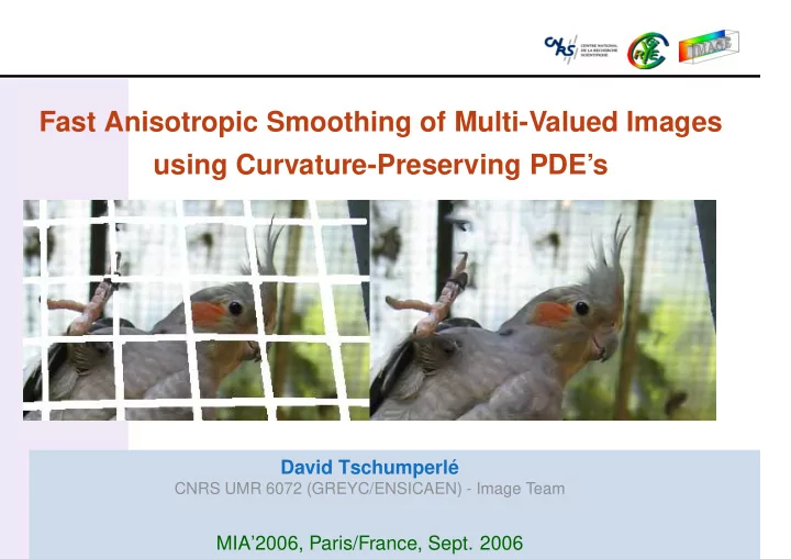
Algorithm properties ⇒ The maximum principle is verified (only local means of pixel intensities are computed). ⇒ Very stable and fast algorithm, compared to classical PDE implementations. The time step ( dt ) can be very large ( ≃ 50 ) while process remains stable. ⇒ LIC-based numerical schemes allows a sub-pixel accuracy for the smoothing ( 4 th - order Runge-Kutta integration) ⇒ Better preservation of small structures. (b) PDE Regul. (a) Original image (c) LIC-base scheme (explicit Euler scheme)