Fast Algorithms Estimating Statistics . . . Applications to Radar . - PowerPoint PPT Presentation
Outline Computing Statistics . . . Interval Uncertainty Fast Algorithms Estimating Statistics . . . Applications to Radar . . . for Computing Statistics Applications to . . . under Interval Uncertainty: Applications to . . . Conclusions
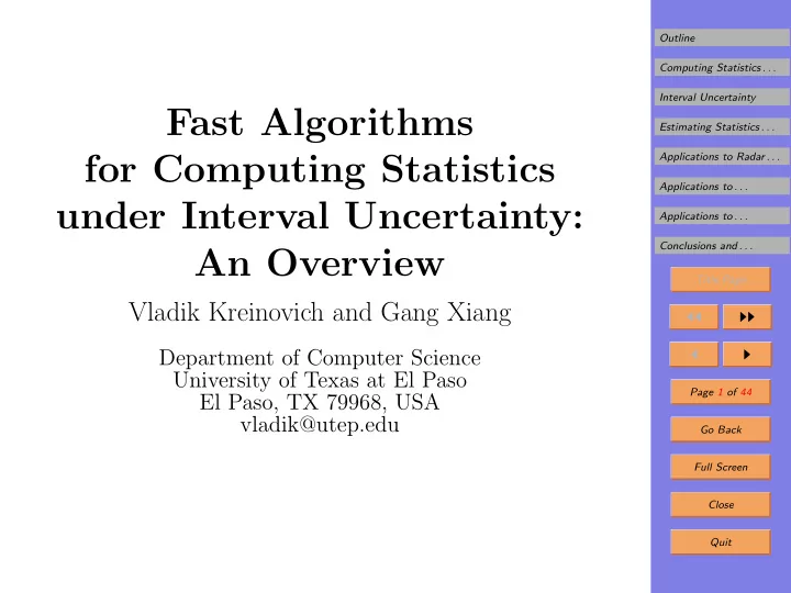
Outline Computing Statistics . . . Interval Uncertainty Fast Algorithms Estimating Statistics . . . Applications to Radar . . . for Computing Statistics Applications to . . . under Interval Uncertainty: Applications to . . . Conclusions and . . . An Overview Title Page Vladik Kreinovich and Gang Xiang ◭◭ ◮◮ Department of Computer Science ◭ ◮ University of Texas at El Paso Page 1 of 44 El Paso, TX 79968, USA vladik@utep.edu Go Back Full Screen Close Quit
Outline 1. Outline Computing Statistics . . . • Formulation of the problem: computing statistics un- Interval Uncertainty der interval uncertainty. Estimating Statistics . . . Applications to Radar . . . • Analysis of the problem. Applications to . . . • Reasonable classes of problems for which we can expect Applications to . . . feasible algorithms for statistics of interval data. Conclusions and . . . • Overview of the classes. Title Page • A sample result: linear algorithm for computing vari- ◭◭ ◮◮ ance under interval uncertainty. ◭ ◮ • Applications. Page 2 of 44 Go Back Full Screen Close Quit
Outline 2. Computing Statistics is Important Computing Statistics . . . • In many engineering applications, we are interested in Interval Uncertainty computing statistics. Estimating Statistics . . . Applications to Radar . . . • Example: we observe a pollution level x ( t ) in a lake at Applications to . . . different moments of time t . Applications to . . . • Objective: estimate standard statistical characteristics: Conclusions and . . . mean E , variance V , correlation w/other measurements. Title Page • For each of these characteristics C , there is an estimate ◭◭ ◮◮ C ( x 1 , . . . , x n ) based on the observed values x 1 , . . . , x n . ◭ ◮ � n • Sample average E ( x 1 , . . . , x n ) = 1 n · x i . Page 3 of 44 i =1 Go Back � n • Sample variance V ( x 1 , . . . , x n ) = 1 ( x i − E ) 2 . n · Full Screen i =1 Close Quit
Outline 3. Interval Uncertainty Computing Statistics . . . • Interval uncertainty in measurements: Interval Uncertainty Estimating Statistics . . . – often, we only know the approximate (measured) Applications to Radar . . . value � x i and the measurement accuracy ∆ i ; Applications to . . . – the actual (unknown) value of x i is in Applications to . . . x i = [ � x i − ∆ i , � x i + ∆ i ] . Conclusions and . . . • Interval uncertainty in observations: Title Page – example: on the 5-th day, the seed did not germi- ◭◭ ◮◮ nate, on the 6-th day it germinated; ◭ ◮ – conclusion: t ∈ [5 , 6]. Page 4 of 44 • Intervals from need to protect privacy: Go Back – instead of recording the exact values of salary, age, Full Screen etc., – we only store the range: e.g., age from 10 to 20, Close from 20 to 30, etc. Quit
Outline 4. Estimating Statistics Under Interval Uncertainty: Computing Statistics . . . A Problem Interval Uncertainty • Situation: in many cases, we only know the intervals Estimating Statistics . . . Applications to Radar . . . x 1 = [ x 1 , x 1 ] , . . . , x n = [ x n , x n ] . Applications to . . . • Problem: different values x i ∈ x i lead to different val- Applications to . . . ues of the statistical characteristic C ( x 1 , . . . , x n ). Conclusions and . . . Title Page • Conclusion: a reasonable estimate for the correspond- ing statistical characteristic is the range ◭◭ ◮◮ def ◭ ◮ = { C ( x 1 , . . . , x n ) | x 1 ∈ x 1 , . . . , x n ∈ x n } . C ( x 1 , . . . , x n ) Page 5 of 44 • Task: modify the existing statistical algorithms so that Go Back they compute these ranges. Full Screen • This is the problem that we will be handling in the Close talk. Quit
Outline 5. Precise Formulation of the Problem: Estimating Computing Statistics . . . Statistics Under Interval Uncertainty Interval Uncertainty • Given: Estimating Statistics . . . Applications to Radar . . . – n intervals x 1 = [ x 1 , x 1 ] , . . . , x n = [ x n , x n ]; Applications to . . . – a statistical characteristic C ( x 1 , . . . , x n ). Applications to . . . • Comment: each interval x i contains the actual (un- Conclusions and . . . known) value x i of the quantity x i . Title Page • Compute: the range ◭◭ ◮◮ def = { C ( x 1 , . . . , x n ) : x 1 ∈ x 1 , . . . , x n ∈ x n } ◭ ◮ C ( x 1 , . . . , x n ) Page 6 of 44 of possible values of C ( x 1 , . . . , x n ) when x i ∈ x i . Go Back Full Screen Close Quit
Outline 6. Analysis of the Problem Computing Statistics . . . • Known fact: for some characteristics, solving this prob- Interval Uncertainty lem is straightforward. Estimating Statistics . . . n � Applications to Radar . . . • Example: the sample mean E = 1 n · x i is monotonic Applications to . . . i =1 Applications to . . . in each of n variables x i . Conclusions and . . . • Conclusion: to find the range [ E, E ] = E ( x 1 , . . . , x n ) , Title Page n n � � we compute E = 1 x i and E = 1 n · n · x i . ◭◭ ◮◮ i =1 i =1 ◭ ◮ • Known fact: for some characteristics, solving this prob- Page 7 of 44 lem is difficult. Go Back • Example: computing the range [ V , V ] = V ( x 1 , . . . , x n ) is, in general, NP-hard. Full Screen Close Quit
Outline 7. Linearization Computing Statistics . . . • General idea: uncertainty comes from measurement er- Interval Uncertainty def rors ∆ x i = � x i − x i (so that x i = � x i − ∆ x i ). Estimating Statistics . . . Applications to Radar . . . • Frequent situation: measurement errors are small. Applications to . . . • Engineering approach: expand C ( x 1 , . . . , x n ) in Taylor Applications to . . . def series at � x i = ( x i + x i ) / 2 and keep only linear terms: Conclusions and . . . n � Title Page C lin ( x 1 , . . . , x n ) = C 0 − C i · ∆ x i , ◭◭ ◮◮ i =1 = ∂C ◭ ◮ def def where C 0 = C ( � x 1 , . . . , � x n ) and C i ( � x 1 , . . . , � x n ) . ∂x i Page 8 of 44 • Resulting estimate: we estimate the range of C as Go Back � n def [ C 0 − ∆ , C 0 + ∆], where ∆ | C i | · ∆ i . = Full Screen i =1 • Shortcoming: the intervals are sometimes wide, so that Close high order terms can no longer be ignored. Quit
Outline 8. Straightforward Interval Computations Computing Statistics . . . • Main idea: inside the computer, every algorithm con- Interval Uncertainty sists of elementary operations f ( a, b ). Estimating Statistics . . . Applications to Radar . . . • Fact: for each f ( a, b ), once we know the intervals a Applications to . . . and b , we can compute the exact range f ( a , b ). Applications to . . . • Straightforward interval computations: replacing each Conclusions and . . . operation f ( a, b ) by the corr. interval operation. Title Page • Known: as a result, we get an enclosure for the desired ◭◭ ◮◮ range. ◭ ◮ • Problem: we get excess width. Example: – For x 1 = x 2 = [0 , 1], the actual V = ( x 1 − x 2 ) 2 Page 9 of 44 and 4 Go Back hence, the actual range V = [0 , 0 . 25]. Full Screen – On the other hand, E = [0 , 1], hence ( x 1 − E ) 2 + ( x 2 − E ) 2 Close = [0 , 1] ⊃ [0 , 0 . 25] . Quit 2
Outline 9. For this Problem, Traditional Optimization Meth- Computing Statistics . . . ods Sometimes Require Unreasonably Long Time Interval Uncertainty • Typical problem: compute the exact range [ V , V ] of the Estimating Statistics . . . finite sample variance. Applications to Radar . . . Applications to . . . • Natural idea: solve this problem as a constrained opti- Applications to . . . mization problem. Conclusions and . . . • Formulation: V → min (or V → max) under the con- Title Page straints ◭◭ ◮◮ x 1 ≤ x 1 ≤ x 1 , . . . , x n ≤ x n ≤ x n . ◭ ◮ • Known: optimization techniques can compute “sharp” Page 10 of 44 (exact) values of min( f ( x )) and max( f ( x )). Go Back • Problem: general constrained optimization algorithms can require exponential time. Full Screen • Difficulty: for n ≈ 300, the value 2 n becomes larger Close than the lifetime of the Universe. Quit
Outline 10. Analysis of the Problem: Summary Computing Statistics . . . • Problem (reminder): compute the range C of a statis- Interval Uncertainty tical characteristic C under interval uncertainty. Estimating Statistics . . . Applications to Radar . . . • Deficiencies of the existing methods: they are Applications to . . . – either not always efficient, Applications to . . . – or do not always provide us with sharp estimates. Conclusions and . . . • Conclusion: we need new methods. Title Page • Main part of our talk: ◭◭ ◮◮ – characteristic: sample variance V ; ◭ ◮ – classes of problems: all previously proposed practi- Page 11 of 44 cally important classes; Go Back – what we do: describe fast methods for computing V for all these classes. Full Screen • Additional results: we describe fast algorithms for sev- Close eral other statistical characteristics. Quit
Recommend
More recommend
Explore More Topics
Stay informed with curated content and fresh updates.
