Fast Algorithms for the Removal of Non-Uniform Motion Blurs James - PowerPoint PPT Presentation
Fast Algorithms for the Removal of Non-Uniform Motion Blurs James G. Nagy Emory University Atlanta, GA Joint work with Julianne Chung, Eldad Haber, John Oshinski Motivating Example Motion in MRI cardiac image Motivating Example Motion in
Fast Algorithms for the Removal of Non-Uniform Motion Blurs James G. Nagy Emory University Atlanta, GA Joint work with Julianne Chung, Eldad Haber, John Oshinski
Motivating Example Motion in MRI cardiac image
Motivating Example Motion in MRI cardiac image Restored MRI cardiac image
Outline • Uniform motion blurs, matrix models • Non-uniform motion blurs, matrix models • Algorithms • Difficulties
Uniform Motion Blur True Image Horizontal Blur Vertical Blur Angled Blur
Uniform Motion Blur True Image Horizontal Blur Vertical Blur Angled Blur
Uniform Motion Blur Linear model: b = A x + n The matrix A is structured: Horizontal blur ⇒ A = T ⊗ I Vertical blur ⇒ A = I ⊗ T 1 d . . . ... 1 where T = d ... 1 1 · · · d d Angled blur ⇒ A = block Toeplitz, Toeplitz blocks
Non-Uniform Motion Blur True Image Non−Uniform Blur
Non-Uniform Motion Blur True Image Non−Uniform Blur
Non-Uniform Motion Blur True Image Non−Uniform Blur We still have linear model b = A x + n However, A has no obvious structure.
Non-Uniform Motion Blur To explicitly construct A : • Estimate direction and magnitude of motion at each pixel • Construct corresponding column of A • Use sparse data structure for A
Sparsity Pattern of A
Sparsity Pattern of A 0 1000 2000 3000 4000 5000 6000 7000 8000 9000 10000 0 1000 2000 3000 4000 5000 6000 7000 8000 9000 10000 nz = 223734
Sparsity Pattern of A 0 100 200 300 400 500 600 700 800 900 1000 0 100 200 300 400 500 600 700 800 900 1000 nz = 13017
Non-Uniform Motion Blur Problem: It may be difficult to estimate motion at every pixel
Non-Uniform Motion Blur To approximate A : • Partition image into regions • Assume motion is uniform in each region • Estimate direction and magnitude of ”uniform” mo- tion in each region • Use interpolation: � A ≈ I k A k where A k is defined by uniform motion in k th region and I k is diagonal, with � I k = I
Region Partitioning One region
Region Partitioning 4 regions
Region Partitioning 9 regions
Region Partitioning 16 regions
Region Partitioning 25 regions
Region Partitioning 64 regions
Deblurring Algorithms Given A (or its approximation), need to solve b = A x + n where • A is ill-conditioned ⇒ need regularization • A is large ⇒ usually need iterative method
Example Singular Value Distribution Horizontal blur Angle blur 0 0 10 10 −2 −2 10 10 −4 −4 10 10 singular values singular values −6 −6 10 10 −8 −8 10 10 −10 −10 10 10 −12 −12 10 10 −14 −14 10 10 −16 −16 10 10 −18 −18 10 10 0 10 20 30 40 50 60 70 80 90 100 110 0 10 20 30 40 50 60 70 80 90 100 110
Deblurring Algorithms Possible regularization methods • Truncated singular value decomposition (TSVD) k u T i b A = U Σ V T � x tsvd = ⇒ v i σ i i =1 (can use efficiently for horizontal or vertical blurs) • Tikhonov: || b − A x || 2 + µ 2 || L x || 2 � � min • Iterative: Terminate iterations early (e.g., conjugate gradients)
Deblurring Algorithms Example of iterative regularization ... 0.65 0.6 relative error 0.55 0.5 0.45 0.4 0.35 0.3 0 5 10 15 20 25 30 35 40 45 iteration
Numerical Examples First consider text data: True Image Non−Uniform Blur • Use CGLS, iterative regularization. • For A , – Approximate motion on regions – Use motion information at every pixel
Numerical Examples Blurred image 0.7 0.6 relative error 0.5 0.4 0.3 0.2 0 10 20 30 40 50 60 70 80 90 100 iteration
Numerical Examples 1 region, 0 iterations 0.7 0.6 relative error 0.5 0.4 0.3 0.2 0 10 20 30 40 50 60 70 80 90 100 iteration
Numerical Examples 4 region, 0 iterations 0.7 0.6 relative error 0.5 0.4 0.3 0.2 0 10 20 30 40 50 60 70 80 90 100 iteration
Numerical Examples 16 region, 1 iterations 0.7 0.6 relative error 0.5 0.4 0.3 0.2 0 10 20 30 40 50 60 70 80 90 100 iteration
Numerical Examples 64 region, 3 iterations 0.7 0.6 relative error 0.5 0.4 0.3 0.2 0 10 20 30 40 50 60 70 80 90 100 iteration
Numerical Examples 256 region, 9 iterations 0.7 0.6 relative error 0.5 0.4 0.3 0.2 0 10 20 30 40 50 60 70 80 90 100 iteration
Numerical Examples 1024 region, 15 iterations 0.7 0.6 relative error 0.5 0.4 0.3 0.2 0 10 20 30 40 50 60 70 80 90 100 iteration
Numerical Examples Every pixel, 79 iterations 0.7 0.6 relative error 0.5 0.4 0.3 0.2 0 10 20 30 40 50 60 70 80 90 100 iteration
Numerical Examples Blurred image 0.2 0.18 0.16 relative error 0.14 0.12 0.1 0.08 0 2 4 6 8 10 12 14 16 18 20 iteration
Numerical Examples 1 region, 1 iterations 0.2 0.18 0.16 relative error 0.14 0.12 0.1 0.08 0 2 4 6 8 10 12 14 16 18 20 iteration
Numerical Examples 4 regions, 1 iteration 0.2 0.18 0.16 relative error 0.14 0.12 0.1 0.08 0 2 4 6 8 10 12 14 16 18 20 iteration
Numerical Examples 16 regions, 3 iterations 0.2 0.18 0.16 relative error 0.14 0.12 0.1 0.08 0 2 4 6 8 10 12 14 16 18 20 iteration
Numerical Examples 64 regions, 7 iterations 0.2 0.18 0.16 relative error 0.14 0.12 0.1 0.08 0 2 4 6 8 10 12 14 16 18 20 iteration
Numerical Examples Every pixel, 14 iterations 0.2 0.18 0.16 relative error 0.14 0.12 0.1 0.08 0 2 4 6 8 10 12 14 16 18 20 iteration
Computational Issues • Choosing a regularization parameter • Fast matrix-vector multiplication should scale well with number of regions • Preconditioning especially when using a lot of regions, or all pixel information • How to get motion information?
Preconditioning • A is ill-conditioned ⇒ preconditioner is ill-conditioned • How to regularize preconditioner? • Relatively easy for circulant, and other transform based preconditioners. • But, A is not well approximated by circulant matrix. • Alternative approach – try: A ≈ C ⊗ D
Preconditioning using Kronecker Products p � Using the model: A = I k A k k =1 • Each A k can be decomposed as: r C ( k ) ⊗ D ( k ) � A k = j j j =1 • Therefore, our model for A is: p r C ( k ) ⊗ D ( k ) � � A = I k j j j =1 k =1
The End! • It is possible to efficiently implement iterative meth- ods for non-uniform motion blurs. • More information provides substantially better restorations. • However, more information results in slower conver- gence of iterative methods. www.mathcs.emory.edu/ ∼ nagy
Recommend
More recommend
Explore More Topics
Stay informed with curated content and fresh updates.

