Factors The characteristics of measurements made under different - PowerPoint PPT Presentation

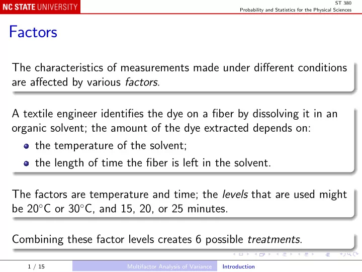
ST 380 Probability and Statistics for the Physical Sciences Factors The characteristics of measurements made under different conditions are affected by various factors . A textile engineer identifies the dye on a fiber by dissolving it in an organic solvent; the amount of the dye extracted depends on: the temperature of the solvent; the length of time the fiber is left in the solvent. The factors are temperature and time; the levels that are used might be 20 ◦ C or 30 ◦ C, and 15, 20, or 25 minutes. Combining these factor levels creates 6 possible treatments . 1 / 15 Multifactor Analysis of Variance Introduction

ST 380 Probability and Statistics for the Physical Sciences Two Factors Example 11.7 The response X is thermal conductivity of asphalt mix (W/(m ◦ K)). The factors are: Asphalt binder grade: PG58, PG64, or PG70. Coarse aggregate content: 38%, 41%, or 44%; In R asphalt <- read.table("Data/Example-11-07.txt", header = TRUE) boxplot(Cond ~ AsphGr, asphalt) boxplot(Cond ~ AggCont, asph) 2 / 15 Multifactor Analysis of Variance Two Factors

ST 380 Probability and Statistics for the Physical Sciences The boxplots show a strong effect of AggCont , and a possible effect of AsphGr . To quantify these impressions, we need to test appropriate null hypotheses. Because both factors may affect the response, the hypotheses must be set up carefully. The hypotheses are defined in the context of a statistical model . 3 / 15 Multifactor Analysis of Variance Two Factors

ST 380 Probability and Statistics for the Physical Sciences Notation Write X i , j , k for: the k th response ( k = 1 or 2) when AsphGr is at level i ( i = 1 , 2 , or 3) and AggCont is at level j ( j = 1 , 2 , or 3) The Additive Model We assume that µ i , j = E ( X i , j , k ) = µ + α i + β j , k = 1 , 2 , for parameters µ , α 1 , α 2 , α 3 , β 1 , β 2 , and β 3 . 4 / 15 Multifactor Analysis of Variance Two Factors

ST 380 Probability and Statistics for the Physical Sciences Estimability The model is over-parametrized as it stands. If a constant c is added to µ and subtracted from each of the α ’s (or from each of the β ’s), the sum remains the same. That is, different sets of parameter values produce the same values for E ( X i , j , k ), so we cannot estimate the parameters. 5 / 15 Multifactor Analysis of Variance Two Factors

ST 380 Probability and Statistics for the Physical Sciences Constraints We can eliminate the nonuniqueness by imposing constraints on the α ’s and β ’s. One possibility, used in the book, is: I J � � α i = β j = 0 . i =1 j =1 Another approach, used in all software, is based on choosing a reference level of each factor. The parameter associated with the reference level is set to zero, which also eliminates the nonuniqueness. 6 / 15 Multifactor Analysis of Variance Two Factors

ST 380 Probability and Statistics for the Physical Sciences In R, the reference level defaults to the first level, while in SAS (and JMP?) the default is the last level: in R: α 1 = β 1 = 0 in SAS: α I = β J = 0 . Note that, in the R convention, µ 1 , 1 = E ( X 1 , 1 , k ) = µ + α 1 + β 1 = µ. That is, in this “reference level” approach, µ is actually the expected response for the treatment in which both factors are at their respective reference levels. 7 / 15 Multifactor Analysis of Variance Two Factors

ST 380 Probability and Statistics for the Physical Sciences Hypotheses The level of the binder grade, AsphGr , has no effect on E ( X ) if α i = 0 , i = 1 , 2 , . . . , I . We test this as a null hypothesis against the alternative that some of the α ’s are nonzero. As in the single-factor case, the usual test statistic is a ratio of mean squares, and is F -distributed under the null hypothesis. A similar statistic tests the null hypothesis that AggCont has no effect: β j = 0 , j = 1 , 2 , . . . , J . 8 / 15 Multifactor Analysis of Variance Two Factors

ST 380 Probability and Statistics for the Physical Sciences In R asphaltAov <- aov(Cond ~ AsphGr + factor(AggCont), asphalt) summary(asphaltAov) Output Df Sum Sq Mean Sq F value Pr(>F) AsphGr 2 0.002089 0.001045 13.7 0.00063 *** factor(AggCont) 2 0.008297 0.004149 54.4 4.83e-07 *** Residuals 13 0.000991 0.000076 --- Signif. codes: 0 *** 0.001 ** 0.01 * 0.05 . 0.1 1 Both factors have very significant effects, especially AggCont . 9 / 15 Multifactor Analysis of Variance Two Factors

ST 380 Probability and Statistics for the Physical Sciences Pairwise Comparisons Knowing that AsphGr has a significant effect on conductivity, the next question is what kind of effect: TukeyHSD(asphaltAov, "AsphGr") Output Tukey multiple comparisons of means 95% family-wise confidence level Fit: aov(formula = Cond ~ AsphGr + factor(AggCont), data = asphalt) $AsphGr diff lwr upr p adj PG64-PG58 0.01166667 -0.001645642 0.024978975 0.0892142 PG70-PG58 -0.01466667 -0.027978975 -0.001354358 0.0306046 PG70-PG64 -0.02633333 -0.039645642 -0.013021025 0.0004494 10 / 15 Multifactor Analysis of Variance Two Factors

ST 380 Probability and Statistics for the Physical Sciences Binder grade PG70 gives significantly lower conductivity than the other grades, but PG58 and PG64 are not significantly different. TukeyHSD(asphaltAov, "factor(AggCont)") shows that all three levels of AggCont give significantly different conductivities. 11 / 15 Multifactor Analysis of Variance Two Factors

ST 380 Probability and Statistics for the Physical Sciences Parameter Estimates When there is only one factor, pairwise comparisons are the most common inferences. We can also estimate the parameters themselves, which will be important when more factors are involved: asphaltLm <- lm(Cond ~ AsphGr + factor(AggCont), asphalt) summary(asphaltLm) 12 / 15 Multifactor Analysis of Variance Two Factors

ST 380 Probability and Statistics for the Physical Sciences Output Call: lm(formula = Cond ~ AsphGr + factor(AggCont), data = asphalt) Residuals: Min 1Q Median 3Q Max -0.011333 -0.004583 -0.001167 0.003583 0.015333 Coefficients: Estimate Std. Error t value Pr(>|t|) (Intercept) 0.841000 0.004602 182.730 < 2e-16 *** AsphGrPG64 0.011667 0.005042 2.314 0.03766 * AsphGrPG70 -0.014667 0.005042 -2.909 0.01219 * factor(AggCont)41 -0.017333 0.005042 -3.438 0.00441 ** factor(AggCont)44 -0.051667 0.005042 -10.248 1.35e-07 *** --- Signif. codes: 0 *** 0.001 ** 0.01 * 0.05 . 0.1 1 13 / 15 Multifactor Analysis of Variance Two Factors

ST 380 Probability and Statistics for the Physical Sciences Output, continued Residual standard error: 0.008732 on 13 degrees of freedom Multiple R-squared: 0.9129, Adjusted R-squared: 0.8861 F-statistic: 34.05 on 4 and 13 DF, p-value: 8.953e-07 Interpretation The “Coefficients” are the estimated parameters: (Intercept) µ ˆ ˆ AsphGrPG64 α 2 AsphGrPG70 α 3 ˆ ˆ factor(AggCont)41 β 2 ˆ factor(AggCont)44 β 3 14 / 15 Multifactor Analysis of Variance Two Factors

ST 380 Probability and Statistics for the Physical Sciences Notes AsphGrPG58 and factor(AggCont)38 are not in the output, because the corresponding parameters α 1 and β 1 are constrained to be zero. Recall that the intercept µ is the expected response for this combination of factor levels. 15 / 15 Multifactor Analysis of Variance Two Factors