Extreme values for diffusion in random media Ivan Corwin Columbia - PowerPoint PPT Presentation
Extreme values for diffusion in random media Ivan Corwin Columbia University From pollen to Perrin History: In 1827, Robert Brown observed that pollen suspended in water seemingly performed a random walk. Eighty years later, Einstein proposed
Extreme values for diffusion in random media Ivan Corwin Columbia University
From pollen to Perrin History: In 1827, Robert Brown observed that pollen suspended in water seemingly performed a random walk. Eighty years later, Einstein proposed a statistical description for this “Brownian motion” and an explanation: Water molecules jiggle and knock the pollen in small and seemingly random di- rections. This model was soon confirmed in experi- ments of Perrin. Questions for today: � Are there senses in which Brownian motion fails to model such a physical system? � Are there signatures of the underlying random media which can be recovered by studying the motion of particles? I will argue that diffusion in random media has very different extreme value statistics / large deviations.
Diffusion in a random media Many small particles moving in a viscous media: � How does the bulk particle density evolve? � What about the right-most particle? Two models for such systems: � Independent random walks. � Independent random walks in a random environment (RWRE). Punchline: Both models have same bulk behavior, but the RWRE dras- tically changes extreme value scalings / statistics to KPZ type.
Case 1: Independent (simple) random walk X t on Z � � � � α β P X t + 1 = X t + 1 = α + β , P X t + 1 = X t − 1 = α + β . � Law of Large Numbers (LLN) : X t → α − β t − α + β . 2 � αβ � Central Limit Theorem (CLT) : For σ = α + β , N (0 , 1) Gaussian, X t − t α − β α + β = ⇒ N (0 , 1) . � σ t � Large Deviation Principle (LDP) : For α − β α + β < x < 1, with � e zX 1 �� � � � I ( x ) = sup z ∈ R zx − λ ( z ) and λ ( z ) : = log ❊ , � �� � log P X t > xt − → − I ( x ) , t � � e.g. For α = β , I ( x ) = 1 (1 + x )log(1 + x ) + (1 − x )log(1 − x ) . 2
Extreme value statistics for random walks � � � � N = P ( X t ≤ x ) N = max( X (1) t ,..., X ( N ) P ) ≤ x 1 − P ( X t > x ) t
Extreme value statistics for random walks � How does the bulk particle density evolve? � What about the right-most particle? Let X (1) t ,... X ( N ) be N -independent copies of X t . Then we have: t � Centered bulk density solves heat equation and is Gaussian. � If N = e ct and c < c saturated , then for c 1 = I − 1 ( c ) (and similarly explicit constants c 2 , c 3 ) � � X ( i ) max ≈ c 1 · t + c 2 · log( t ) + c 3 · Gumbel t i = 1 ,..., N where Gumbel has distribution function e − e − x .
Deriving exact formulas via a recurrence n Z ( t , n ) X t t 0 x (0 , 1) t Recurrence formula Define a function Z ( t , n ) via the recursion (with Z (0 , n ) = 1 n ≥ 1 ) α β Z ( t , n ) = α + β · Z ( t − 1 , n ) + α + β · Z ( t − 1 , n − 1) . We have equality of � � Z ( t , n ) = P X t � t − 2 n + 2 . This recursion is easily solved in terms of Binomial coefficients.
Asymptotics via contour integrals Binomial coefficients can be written in terms of contour integrals: � � � n = 1 (1 + z ) n z − k dz z . k 2 π i | z |< 1 Can study various asymptotic regimes for n and k . � � � n = 1 e nf ( z ) dz f ( z ) = log(1 + z ) − 1 z , with 2 log z . n /2 2 π i | z |< 1 Steepest descent analysis expands around f ( z )’s critical point z = 1.
Case 2: Random walks in random environment (RWRE) Let B = ( B t , x ) t , x be independent random variables with a common fixed distribution on [0 , 1]. Call P the probability measure on B . For a given instance of B let P B denote the probability measure on sim- ple random walks on Z with left / right jump probabilities � � � � � � � X t = x � X t = x P B X t + 1 = x + 1 = B t , x , P B X t + 1 = x − 1 = 1 − B t , x . Consider independent P B -distributed copies X (1) t ,..., X ( N ) of X t . t X t t 0 x Bt , x ( t , x ) 1 − Bt , x
CLT and LDP Theorem (Rassoul-Agha and Seppäläinen, 2004) � � � � � 1 − v 2 . Assume P 0 < B t , x < 1 > 0 and let v = 2 E B t , x − 1 and σ = Then for P -almost every choice of jump rates, X ⌊ nt ⌋ −⌊ nt ⌋ v as a process in t − − − − − − − − − − − → BM ( t ) . σ � n n →∞ Theorem (Rassoul-Agha, Seppäläinen and Yilmaz, 2013) � e zX t �� �� � 3 � � < ∞ . Then λ ( z ) : = lim t →∞ 1 Assume E log( B t , x ) t log ❊ B exists and is constant P -almost surely. For I ( x ) the Legendre transform of λ ( z ) � �� � log P B X t > xt P − almost surely − − − − − − − − − − − → − I ( x ) . t t →∞ � Finding an explicit formula for λ ( z ) or I ( x ) is generally not possible. � Random rate I ( x ) ≥ deterministic rate I ( x ) (by Jensen’s inequality). � � � Lower order fluctuations of P B X t > xt are lost in this result.
Integrable probability to the rescue In a lab, how could we distinguish deterministic or random media? � × Extreme value speed depends non-universally on the underlying random walk model or media. � � Extreme value fluctuations have different behaviors than in the deterministic and random cases. (See below!) Definition The Beta RWRE has Beta ( α , β )-distributed jump probabilities B t , x : � � = y α − 1 (1 − y ) β − 1 Γ ( α + β ) P B t , x ∈ [ y , y + d y ] Γ ( α ) Γ ( β )d y . If α = β = 1, we recover the uniform distribution on [0 , 1]. Aim We will show how to compute the distribution of P B ( X t ≥ x ) exactly.
Large deviations and cube-root fluctuations For simplicity lets take α = β = 1 (i.e. B t , x uniform on [0 , 1]). Theorem (Barraquand-C ’15) For B t , x uniform on [0 , 1] , the large deviation principle rate function is � �� � log P B X t > xt � 1 − x 2 . lim = I ( x ) = 1 − t →∞ − t Moreover, as t → ∞ , we have convergence in distribution of � �� � log P B X t > xt + I ( x ) t = ⇒ L GUE , σ ( x ) · t 1/3 where L GUE is the GUE Tracy-Widom distribution, and σ ( x ) 3 = 2 I ( x ) 2 1 − I ( x ) . Cube-root L GUE fluctuations are a hallmark of random matrix theory and the Kardar-Parisi-Zhang universality class.
Extreme value fluctuations Corollary (Barraquand-C ’15) For B t , x uniform on [0 , 1] , let X (1) t ,..., X ( N ) be random walks drawn t independently according to P B . For N = e ct with c ∈ (0 , 1) , � � � X ( i ) max N 1 − (1 − c ) 2 − t t i = 1 = ⇒ L GUE . d ( c ) · t 1/3 Compare max r(andom probabilities) to max d(eterministic probabilities) : � max r has a slower speed than max d (the random B t , x routes many walkers along the same path and hence decreases entropy). � max r fluctuates O ( t 1/3 ) versus O (1) for max d .
Diffusion in a (random) media Many small particles moving in a viscous media: � How does the bulk particle density evolve? � What about the right-most particle? Two models for such systems: � Independent random walks. � Independent random walks in a random environment (RWRE). Punchline: Both models have same bulk behavior, but the RWRE dras- tically changes extreme value scalings / statistics to KPZ type.
Walking across a city (the α , β → 0 limit) � For every edge, let E e be i.i.d. exp(1) and for each vertex ξ i , j i.i.d. Bernoulli(1/2). � Define the passage time of an edge D n , m � m ξ i , j E e if vertical ( i , j ) → ( i , j + 1) , t e = (1 − ξ i , j ) E e if horizontal ( i , j ) → ( i + 1 , j ) . � Define the first passage-time T ( n , m ) from (0 , 0) to the half-line D n , m by � T ( n , m ) = min t e . π :(0 , 0) → D n , m (0 , 0) e ∈ π n Theorem For any κ > 1 , there are explicit functions ρ ( κ ) and τ ( κ ) such that T ( n , κ n ) − τ ( κ ) n = ⇒ L GUE . ρ ( κ ) n 1/3
Dynamical construction of percolation cluster Alternative description � At time 0, only one random walk trajectory (in black). � From each point in the cluster, at exponential rate one we add the trace of a new random walk (until it rejoins the cluster). � Colors represent when a point joined the cluster. Barraquand-Rychnovsky ’18 Prove a limit theorem for the shape of the percolation cone and that its fluctuations have a 4/9 exponent!
Sticky Brownian motion (another α , β → 0 limit) Brownian motion sticky at the origin (Feller ’52): Random walk away from origin; at origin, escape with probability n − 1/2 A pair of sticky Brownian motions has difference sticky at the origin. N -particle sticky Brownian motion : Diffusive limit of N particles in the same random environment, when the B t , x are close to 0 or 1. Need to specify rate for clusters of k + ℓ particles to “split” into separate clusters of size k and ℓ . Rate for limit of Beta RWRE is k + ℓ k ℓ . Barraquand- Rychnovsky ’19 prove KPZ extreme value results for this model.
Recommend
More recommend
Explore More Topics
Stay informed with curated content and fresh updates.
