Example: How to Train Interval Predictor Models 7th SIPTA Summer - PDF document

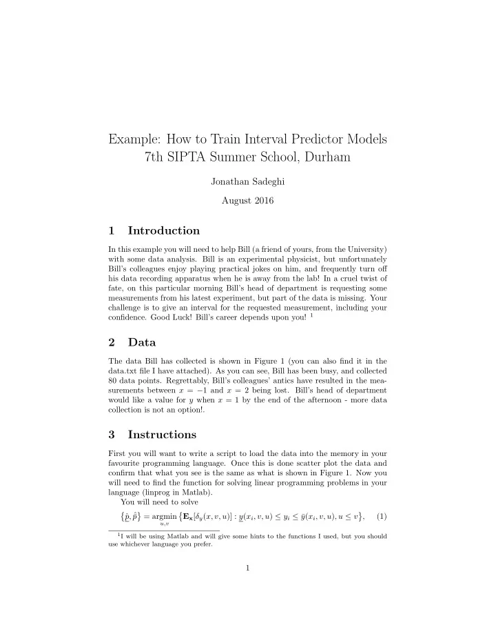
Example: How to Train Interval Predictor Models 7th SIPTA Summer School, Durham Jonathan Sadeghi August 2016 1 Introduction In this example you will need to help Bill (a friend of yours, from the University) with some data analysis. Bill is an experimental physicist, but unfortunately Bill’s colleagues enjoy playing practical jokes on him, and frequently turn off his data recording apparatus when he is away from the lab! In a cruel twist of fate, on this particular morning Bill’s head of department is requesting some measurements from his latest experiment, but part of the data is missing. Your challenge is to give an interval for the requested measurement, including your confidence. Good Luck! Bill’s career depends upon you! 1 2 Data The data Bill has collected is shown in Figure 1 (you can also find it in the data.txt file I have attached). As you can see, Bill has been busy, and collected 80 data points. Regrettably, Bill’s colleagues’ antics have resulted in the mea- surements between x = − 1 and x = 2 being lost. Bill’s head of department would like a value for y when x = 1 by the end of the afternoon - more data collection is not an option!. 3 Instructions First you will want to write a script to load the data into the memory in your favourite programming language. Once this is done scatter plot the data and confirm that what you see is the same as what is shown in Figure 1. Now you will need to find the function for solving linear programming problems in your language (linprog in Matlab). You will need to solve � p, ˆ � � � ˆ ¯ = argmin E x [ δ y ( x, v, u )] : y ( x i , v, u ) ≤ y i ≤ ¯ y ( x i , v, u ) , u ≤ v (1) p , u,v 1 I will be using Matlab and will give some hints to the functions I used, but you should use whichever language you prefer. 1

30 20 y 10 0 − 4 − 2 0 2 4 x Figure 1: Bill’s Data where x i and y i are your data points, ¯ y and y are the bounds for the IPM, ¯ p and p are the parameters you need to find for your IPM and δ y ( x, v, u ) is the spread of the IPM. To simplify your program I would recommend using the sample mean for E x . If you are using Matlab you should compute 3 things 2 : • f : A vector which when multiplied by your parameters vector 3 gives the objective function. • A : A matrix which when multiplied by your parameters vector gives the upper and lower bounds to your IPM as a vector. • b : A vector containing your data points ( y ) 4 . For all three you will require a basis ( φ ( x )), and for simplicity I recommend choosing a polynomial basis. The degree of the polynomial is your choice, but degree 2 seems to be a good place to start. Note that you will also need to extend A and b to include some extra constraints to ensure that ¯ p > p , but this should be trivial. The next section contains the formulae you will need. 4 Useful Formulae The lower bound of the IPM is given by � φ ( x ) − | φ ( x ) | � � φ ( x ) + | φ ( x ) | � p T + p T y ( x, ¯ p, p ) = ¯ (2) , 2 2 2 See http://uk.mathworks.com/help/optim/ug/linprog.html for info on what is required for linear optimisation in Matlab. I will use the default Matlab symbols given on that page. 3 Hint: you should join ¯ p and p into one vector (called x on the Matlab page). 4 Note: for A and b you should ensure you choose appropriate signs to flip the inequality symbol when necessary. 2

and the upper bound is given by � φ ( x ) + | φ ( x ) | � � φ ( x ) − | φ ( x ) | � p T + p T y ( x, ¯ ¯ p, p ) = ¯ . (3) 2 2 The spread of the IPM is given by p − p ) T | φ ( x ) | . δ y ( x, ¯ p, p ) = (¯ (4) 5 Reliability If all has gone well you should now have a well trained IPM at your disposal. But Bill is not safe yet! Write down the interval for x = 1, and save a plot of the IPM for later. Now you must find the reliability of your predictions (i.e. the probability that an unseen measurement of y could fall outside the interval you have given). R , the reliability of the IPM, is bounded by P ( R ≥ 1 − ǫ ) ≥ 1 − β, (5) for reliability parameter ǫ and confidence parameter β satisfying � k + d − 1 � k + d − 1 � N � ǫ i (1 − ǫ ) N − i ≤ β, � (6) k i i =0 where you have used N data points to train the IPM, discarded k data points ( k = 0 for you, unless you have added an outlier removal algorithm) and d is the number of optimisation parameters you used (twice the length of ¯ p ). You may now do two things. Either produce a plot of 1 − β against 1 − ǫ or attempt to find 1 − ǫ for a suitably high confidence (1 − β = 10 − 5 or 1 − β = 10 − 10 , for example). There are many ways to achieve either of these. For the plot you could try a loop or something more complicated. For the high confidence value of reliability you could use something like the fzero function in Matlab. 6 Answers Using a degree 2 IPM I obtained 3 . 1696 > y > − 1 . 9732 and 0 . 8443 > R with confidence greater than 0 . 99. If you would like to see a plot of the confidence interval from the original function or my solution in Matlab please ask! Interesting questions: How many more data points does Bill require to reach a reliability of 0 . 99 with near certainty? How does this result change depending upon the degree of the IPM used? 3