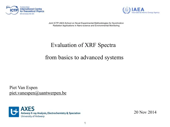
Evaluation of XRF Spectra from basics to advanced systems Piet Van - - PowerPoint PPT Presentation

1

Evaluation of XRF Spectra from basics to advanced systems

Joint ICTP-IAEA School on Novel Experimental Methodologies for Synchrotron Radiation Applications in Nano-science and Environmental Monitoring

Piet Van Espen piet.vanespen@uantwerpen.be

20 Nov 2014

2

Content

• 1. Introduction: some concepts
• 2. Simple peak integration
• 3. Method of least squares
• 4. Fitting of x-ray spectra
• 5. Improvements to the model
• 6. Final remarks

3

Some basic concepts

Nature and science: a personal view Nature = Signal + Noise Science = Model + Statistics

4

4

Why spectrum evaluation? element concentrations ⇔ net intensity of fluorescence lines But: frequent peak overlap presence of a continuum Especially in energy-dispersive spectra

interference free continuum corrected

5

Spectrum contains

• Information: energy and intensity of x-rays

• Amplitude noise: due to Poisson statistics


► fluctuations in the spectrum


• Energy noise: finite resolution of the detector

► nearly Gaussian peaks with a width of ~160 eV

Information content of a spectrum the signal the noise

6

Amplitude noise

Counting events involves Poisson statistics Poisson probability density function: The probability to observe N counts if the true number is µ

Poisson : P(N | µ=3) Normal : P(x | µ=3 σ2 = 3)

Property:

Poisson distribution µ ≅ Normal distribution µ and σ2 = µ approximation is very good for µ (or N) ≥ 9

7

Resolution of ED-XRF spectrometers

Full Width at Half Maximum (FWHM) of a peak Mn Kα @ 5.895 keV FWHMDet = 120 eV FWHMElec = 100 eV => FWHMPeak = 156 eV Intrinsic contribution

2.35 √ × F × E

ϵ energy to create e-h pair 3.85 eV F Fano factor ~0.114 E x-ray energy in eV

FWHM2

Peak = FWHM2 Elec + FWHM2 Det

Electronic noise ~100 eV Energy Noise

8

Cr – Mn – Fe overlap at ~20 eV Cr – Mn – Fe overlap at ~160 eV Resolution of ED-XRF spectrometers

Energy Noise

9

Without amplitude noise (counting statistics) there would be NO PROBLEM

But it is part of the nature We can only measure longer or with a more efficient system

Without energy noise there would be LITTLE PROBLEM

The natural line width of x-rays is only a few eV!!! The observed peak width is the result of the detection process with a fundamental limitation imposed by the Fano factor

10

10

Information content of a spectrum If no energy noise or no amplitude noise ► could determine the “information” unambiguously Need methods to extract information in a optimum way These methods rely on “addition” information (knowledge)
 to extract the useful information Not the method itself is important (if implemented correctly)
 but the correctness of the additional information.

11

• 2. Simple peak integration

12

Simple peak integration Estimate Uncertainty We have to make assumptions integration limits linear background no interference As good as is can get if the assumptions (model) are correct!

13

• 3. Method of Least Squares

14

Need to “estimate” the net peak area with highest possible

• correctness (no systematic error)
• precision (smallest random error)

Least-squares estimation (fitting):

• unbiased
• minimum variance

Limiting factors:

• counting statistical fluctuations (precision)
• accuracy of the fitting model

Method of least squares

15

Method of least squares, straight line

SS = X

i

[yi − y(i)]2 = X

i

[yi − b0 − b1xi]2 = min

⇤SS ⇤b0 = 0 → X

i

yi = b0n + b1 X

i

xi ⇤SS ⇤b1 = 0 → X

i

xiyi = b0 X xi + b1 X

i

x2

i

Set of 2 equations in 2 unknowns b0 and b1 Normal equations

Direct analytical solution Data: {xi,yi}, i=1, 2, …, N Model: y(i) = b0 + b1xi Fitting the model: estimating b0 and b1 Criterion: noise

16

• 4. Fitting X-ray Spectra

17

Least-squares estimate of x-ray spectrum parameters

Peak described by a Gaussian Minimum: No direct analytical solution Search χ2 for minimum

2 = 1 ⌫

n2

X

i=n1

1 wi [y(i) − yi]2

y(i) = b + A 1 σ √ 2π exp (xi − xp)2 2σ2

• position

width area continuum

Criterion, agreement between model and data

linear parameter non-linear

18

We can still apply the concept of least squares minimising the square of the differences between the model and the data The sum of squares is a function of the values of the parameters and for a given set of values should be minimum In this case SS describes a 4 dimensional hyper-surface in a 5- dimension space h We can only “see” in 3-dimensions but mathematically we can search in a higher dimensional space to locate the minimum Starting from some initial values we can modify the parameter values until the minimum is reached. χ2 = χ2(b, h, x0, w) = 1

ν

P

i 1 yi [yi − y(xi, b, h, x0, w)]2

w

19

General form of such a search algorithm

• 1. Select starting values for all parameters bj

and calculate the ch-square

• 2. Obtain (calculate, guess...) a change

(increment or decrement) Δbj such that one moves towards the minimum:

• 3. Replace the old parameter values with the new ones


b ← b + Δb

• 4. repeat step 2 until the “true” minimum is found

Iterative process

AXIL = Analysis of X-ray spectra by Iterative Least-squares

χ = χ(b) χ(b + ∆b) < χ(b)

20

Analytically important parameters: net peak areas In general y(i) is non-linear → Marquardt – Leverberg algorithm Gradient search ↔ linearisation Reliable error estimated But unstable Statistical optimal estimate: using correct weight (Poisson statistics wi = yi)

2 = 1 ⌫

n2

X

i=n1

1 wi [y(i) − yi]2

21

10 peaks ⇒ > 30 parameters !!!! WANT WORK in practice!!!! But we can do better

⇒ Add additional information to the model We known the energies of the x-ray lines (in most cases) Where they are depends on the energy calibration (the same applies to the width of the peaks: resolution calibration)

G(i, E) = Gain σ(E) √ 2π exp (Ei − E)2 2σ2(E)

• Gaussian peak shape

Energy relation: Resolution relation: E(i) = Zero + Gain × i

(E) = "✓ Noise 2 √ 2 ln 2 ◆2 + ✏FanoE #1/2

Only 4 non-linear parameters For 10 peaks only 14 parameters

Need parsimony!!!

22

Already better, but we know more

We know (to some extend) the ratio between lines of an element

IKα2 IKα1 , IKβ IKα . . .

We can group lines together (“peakgroup”) with one “area” and fixed intensity ratios

Continuum function Area Line ratio Peak shape

for j elements (or peak groups)

y(i) = yCont(i) + X

j

Aj (X

k

RjkP(i, Ejk) )

10 elements ⇒ 10 Area’s + 4 calibration parameters

23

Further refinements: escape peaks

Known position (energy) intensity (escape probability)

24

Sum peaks

Known position relative intensity

25

And more

Different background models polynomial exponential polynomial Bremsstrahlung background filter background Parameter constraining

and more...

26

27

Highly flexible method

• Fit individual lines, multiplets, elements…
• Different parametric and non-parametric continuum models
• Include escape and sum peaks

Quality criteria

• Chi-square of fit
• uncertainty estimate of parameters

Statistically correct

• unbiased, minimum variance estimate of the parameters

“Resolving power” is only limited by the noise (counting statistic) BUT THE MODEL MUST BE ACCURATE

28

• 5. Improvements to the model

29

Incorrectness of the model

Not all peaks follow the energy calibration relation

• incoherent (Compton) scatter peaks
• spurious peaks (diffraction, γ-rays)
• even the relation might not be linear

Not all peaks follow the resolution calibration relation

• incoherent scatter peaks (are wider)
• spurious peaks

Peaks are certainly not perfect Gaussians

• shelf (step) due to detector effects (incomplete charge collection)
• tailing due to radiative effects and detector effects
• deviation due to natural line width (Lorentzian)

30

Incorrect fitting model biased results

Solution Adapt the model
 (fitting region, which lines to include...)
 for each particular case Very inconvenient
 when analyzing many spectra

⇒

especially for trace elements

31

Step

h i S(i, Ejk) = Gain 2Ejk erfc E(i) − Ejk

• √

2

• Peak

P(i, Ejk) = G(i, Ejk) + fSS(i, Ejk) + fT T(i, Ejk)

Adding 1 non-linear and 2 linear parameters for each peak!!! Tail

T(i, Ejk) = Gain 2 exp h − 1

2β2

i exp E(i) − Ejk

• erfc

E(i) − Ejk

• √

2 + 1 √2

• Improve the peak profile

Where is my parsimony gone!!! Improvements

32

Step parameterisation

Step is a fundamental aspect of the detector
 (charge loss by photo-electrons near the surface of the detector)

Step fraction fS is related to the MAC

• f the detector crystal

Tail fraction parameterisation

Tail fraction fT is related to the MAC of the detector and the type

• f radiation (Kα and Kβ)

The tail has a component due to the detector and a radiative component

33

Tail width parameterisation

similar magnitude over the entire energy range fS(Ejk) = µDet(Ejk) (a0 + a1Ejk) fTKα(Ejk) = b0 + b1µDet(Ejk) fTKβ(Ejk) = c0 + c1µDet(Ejk) (Ejk) = d0 + d1Ejk

(compare to Zero, Gain, Noise and Fano)

⇒ Fitting parameters a0, a1, b0, b1, c0, c1, d0, d1

34

improvement

Fit of a NIST SRM 1106 Brass spectrum (SpecTrace 5000, Rh tube)

35

To account for peak shift and peak broadening

Need to make the peak profile still a bit more complicated X X G ( i , E ) = G a i n

• (

E ) √ 2 ⇡ e x p  ( E

i

− E ( i ) +

• E

)

2

2

• 2

( E )

• γ peak broadening parameter (normally 1.00)

δE peak shift parameter (normally 0.00) These parameters are constrained to vary within a certain range Eini − ∆E ≤ E ≤ Eini + ∆E ini − ∆ ≤ ≤ ini + ∆

36

The last step

Replace Gaussian with the convolution of a Gaussian with a Lorentzian = Voigt profile

Gain jk √ 2⇡K E(i) − Ejk jk √ 2 , ↵L 2jk √ 2 !

K(x, y) = Re ⇥ exp(−z2)erfc(−iz) ⇤ z = x + iy

with K(...) the complex error function For high Z elements the natural line width becomes substantial relative to the detector resolution

37

Natural line width at high Z elements becomes important e.g. W K ~ 50 eV Gaussians Voigts

38

Original fit of a geological standard (JG1)

39

Improved fit of the geological standard (JG1) Mo secondary target No background

40

NIST SRM 1155

41

NIST SRM 1247

42

More Details Handbook of X-ray Spectrometry

• R. Van Grieken, A. Markowicz

Marcel Decker, N.Y. 2002 ISBN: 0-8247-0600-5 Chapter 4: Spectrum Evaluation

43

Some final remarks: The future Non-linear least-squares works if you have a good parsimonious model if you have TIME X-ray fluorescence imaging: 256 x 256 image = 65536 x-ray spectra @ 1 s / spectrum = 65536 seconds = 1092 minutes = 18 hours !!!! Need to explore new methods Linear models? Multivariate models?

44

• 6. Final remarks

45

Thanks for your attention