Estimation of moment-based models with latent variables work in - PowerPoint PPT Presentation

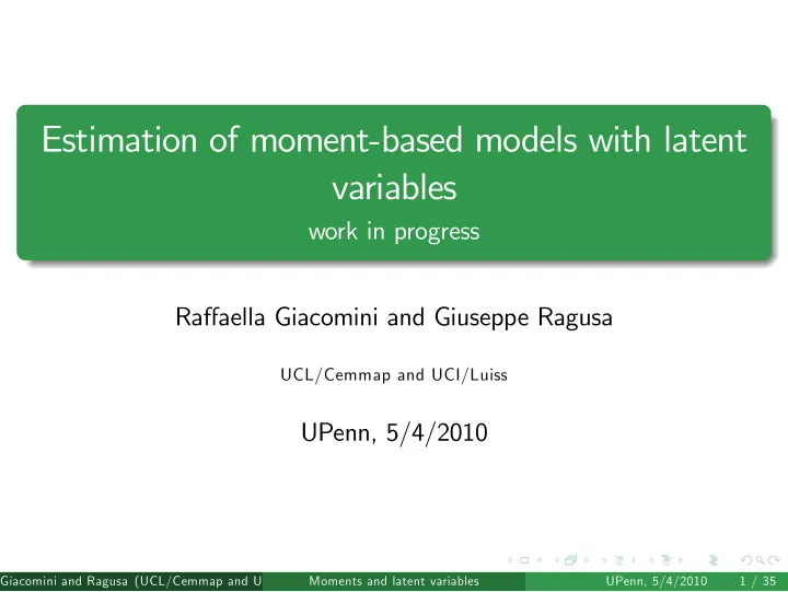
Estimation of moment-based models with latent variables work in progress Ra¤aella Giacomini and Giuseppe Ragusa UCL/Cemmap and UCI/Luiss UPenn, 5/4/2010 Giacomini and Ragusa (UCL/Cemmap and UCI/Luiss) Moments and latent variables UPenn, 5/4/2010 1 / 35

Dynamic latent variables in macroeconomic models E.g., time-varying parameters, structural shocks, stochastic volatility etc. Typical parametric setting: X T = ( X 1 , ..., X T ) = ( Y T , Z T ) , Y T observable, Z T latent Joint density p ( X , θ 0 ) = p ( Y T j Z T , θ 0 ) p ( Z T , θ 0 ) = ) estimation of θ 0 based on integrated likelihood Z p ( Y T j Z T , θ ) p ( Z T , θ ) dZ T b θ = arg max θ Integrated likelihood computed by state-space methods Giacomini and Ragusa (UCL/Cemmap and UCI/Luiss) Moments and latent variables UPenn, 5/4/2010 2 / 35

Existing state-space methods State equation ! p ( Z T , θ ) known in closed form Observation equation ! p ( Y T j Z T , θ ) "…ltering" density known in closed form (e.g. Kalman …lter) or easy to simulate Integral can be computed by MCMC methods Giacomini and Ragusa (UCL/Cemmap and UCI/Luiss) Moments and latent variables UPenn, 5/4/2010 3 / 35

State-space methods for limited information models? We consider the following scenario: p ( Z T , θ ) known ! state equation same as before p ( Y T j Z T , θ ) unknown. Only information about θ is in the form of (non-linear) moment conditions E t � 1 [ g ( Y t , Z t , θ )] = 0 ! substitute observation equation with moment conditions Giacomini and Ragusa (UCL/Cemmap and UCI/Luiss) Moments and latent variables UPenn, 5/4/2010 4 / 35

Applications. GMM with time-varying parameters Example #1. Time-varying "structural" parameters: E [ g ( Y t , β t )] = 0 β t = Φ β t � 1 + ε t , ε t � iidN ( 0 , Σ ) E [ � ] de…ned with respect to joint distribution of Y t and β t Want to estimate θ = ( Φ , Σ ) and sequence of "smoothed" β t Application: Cogley and Sbordone’s (2005) analysis of stability of structural parameters in a Calvo model of in‡ation Giacomini and Ragusa (UCL/Cemmap and UCI/Luiss) Moments and latent variables UPenn, 5/4/2010 5 / 35

Applications. "Robust" stochastic volatility estimation Example #2. Y t = σ t ε t � � = α + β log � � + v t , v t � iidN ( 0 , 1 ) σ 2 σ 2 log t � 1 t Existing estimation methods require distributional assumption on ε t (typically N ( 0 , 1 ) ) Problem: does not capture "fat tails" of …nancial data = ) include jumps or use fat-tailed distribution for ε t (not as straightforward as in GARCH case) Our method is robust to misspeci…cation in distribution of ε t Giacomini and Ragusa (UCL/Cemmap and UCI/Luiss) Moments and latent variables UPenn, 5/4/2010 6 / 35

Applications. Nonlinear DSGE models Example #3. Prototypical DSGE model. Optimality conditions: E t � 1 [ m ( Y t , S t , Z t , β )] = 0 S t = f ( S t � 1 , Y t , Z t , β ) Φ Z t � 1 + ε t , ε t � iidN ( 0 , Σ ) Z t = Want to estimate θ = ( β , Φ , Σ ) Y t = observable variables S t = endogenous latent variables Z t = exogenous latent variables m ( � ) and f ( � ) known Giacomini and Ragusa (UCL/Cemmap and UCI/Luiss) Moments and latent variables UPenn, 5/4/2010 7 / 35

An and Schorfheide (2007) DSGE model In AS model, the endogenous latent variable equation has a simple form: S t = f ( Y t , Z t , β ) (1) Can substitute S t and rewrite the equilibrium conditions as E t � 1 [ g ( Y t , Z t , β )] = 0 Z t = Φ Z t � 1 + ε t , ε t � iid N ( 0 , Σ ) Warning: not all DSGEs …t this framework Giacomini and Ragusa (UCL/Cemmap and UCI/Luiss) Moments and latent variables UPenn, 5/4/2010 8 / 35

Existing approaches to estimation of DSGE models Theory does not provide likelihood � ! must use approximation 1 methods Linearize around steady state (Smets and Wouters, 2003; 2 Woodford, 2003) Solve the model to …nd policy functions Y t = h ( S t , Z t ) Construct likelihood by Kalman …lter Nonlinear approximations (Fernandez-Villaverde and 3 Rubio-Ramirez, 2005) Solve the model (numerically or analytically in the case of second order approximations around steady state) to …nd policy functions Construct likelihood by nonlinear state-space methods (e.g., particle …lter) Giacomini and Ragusa (UCL/Cemmap and UCI/Luiss) Moments and latent variables UPenn, 5/4/2010 9 / 35

Drawbacks of existing likelihood-based approaches Linearization = possible loss of information 1 (Fernandez-Villaverde and Rubio-Ramirez, 2005) Must impose structure to solve the model 2 Add "shocks"/measurement error to avoid stochastic singularity 1 Restrict parameters to rule out indeterminacy (multiple rational 2 expectations solutions) Nonlinear state-space methods computationally intensive (must 3 solve the model for each parameter draw) = ) so far mostly applied to simple models Giacomini and Ragusa (UCL/Cemmap and UCI/Luiss) Moments and latent variables UPenn, 5/4/2010 10 / 35

Relationship with simulation-based method of moments GMM, SMM, EMM, Indirect inference (eg, Ruge-Murcia, 2010) Di¤erence: requires knowledge of p ( Y T j Z T ) or focuses on moments of the type E Y [ g ( Y , β )] = 0 , (2) where g ( Y , β ) can be computed by simulation In our case, the model gives E Y , Z [ m ( Y , Z , β )] = 0 = ) can be written as (2) only if p ( Z j Y ) known Unlike these methods, we directly obtain estimates of the smoothed latent variables Giacomini and Ragusa (UCL/Cemmap and UCI/Luiss) Moments and latent variables UPenn, 5/4/2010 11 / 35

The idea Propose methods for estimating non-linear moment-based models that "exploit" the information contained in the moment conditions Methods are: Computationally convenient 1 Classical or Bayesian 2 Giacomini and Ragusa (UCL/Cemmap and UCI/Luiss) Moments and latent variables UPenn, 5/4/2010 12 / 35

Key elements of methodology Recall problem we want to solve (e.g., classical framework) Z p ( Y T j Z T , θ ) � p ( Z T , θ ) dZ T max θ " unknown " known Two steps: Approximate the unknown likelihood p ( Y T j Z T , θ ) 1 Integrate out the latent variables using classical or Bayesian 2 methods For DSGEs: from an exact likelihood of the approximate 3 model.... to an approximate likelihood of the exact model Giacomini and Ragusa (UCL/Cemmap and UCI/Luiss) Moments and latent variables UPenn, 5/4/2010 13 / 35

Approximate likelihoods We consider two di¤erent approximation strategies Both use projection theory (for no latent variables, Kim (2002), Chernozhukov and Hong (2003), Ragusa (2009)): out of all probability measures satisfying the moment conditions, choose the one that minimizes the Kullback-Leibler information distance Method 1 does not require solving the model (but not applicable to models with dynamic latent endogenous variables) Method 2 applicable to all models but requires solution of (approximate) model Giacomini and Ragusa (UCL/Cemmap and UCI/Luiss) Moments and latent variables UPenn, 5/4/2010 14 / 35

Approximate likelihoods - Method 1 Find density that satis…es moment conditions and minimizes distance from the true density: gives approximate likelihood p ( Y T j Z T , θ ) ∝ e � �� � � � � � � 1 Y T , Z T , θ Y T , Z T , θ Y T , Z T , θ 2 g 0 V � 1 exp g T T T � � T 1 Z T , θ ∑ p g T = g ( Y t , Z t , θ ) � w t � 1 T t = 1 � � � � Y T , Z T , θ Y T , Z T , θ V T = Var ( g T ) , w t � 1 instruments Giacomini and Ragusa (UCL/Cemmap and UCI/Luiss) Moments and latent variables UPenn, 5/4/2010 15 / 35

Approximate likelihoods - Method 1 p ( Y T j Z T , θ ) ∝ e � �� � � � � � � 1 Y T , Z T , θ Y T , Z T , θ Y T , Z T , θ 2 g 0 V � 1 exp g T T T p ( Y T j Z T , θ ) is a simple transformation of the GMM objective e function. Intuition: � � � 0 When ( Z T , θ ) is consistent with the model g T Y T , Z T , θ p ( Y T j Z T , θ ) close to max value of 1. ) e = When ( Z T , θ ) is inconsistent with the moment conditions = ) large values of � � � � � � = Y T , Z T , θ Y T , Z T , θ Y T , Z T , θ V � 1 g 0 g T ) T T p ( Y T j Z T , θ ) � 0. e Giacomini and Ragusa (UCL/Cemmap and UCI/Luiss) Moments and latent variables UPenn, 5/4/2010 16 / 35

Approximate likelihoods - Method 2 Write p ( Y T j Z T ) = Π T t = 1 p ( Y t j Z t , Y t � 1 ) p ( Y t j Z t , Y t � 1 , θ ) (does not need Choose approximate density b to satisfy moment condition but easy to calculate) - For DSGEs, e.g., linearize model around steady state and apply p ( Y t j Z t , Y t � 1 , θ ) are the …ltered densities ) b Kalman …lter = Giacomini and Ragusa (UCL/Cemmap and UCI/Luiss) Moments and latent variables UPenn, 5/4/2010 17 / 35

Approximate likelihoods - Method 2 p ( Y t j Z t , Y t � 1 , θ ) towards moment condition "Tilt" b E t � 1 [ g ( Y t , Z t , θ )] = 0 , new density e p ( � ) satis…es moment condition and minimizes Kullback Leibler distance from b p ( � ) : Solve problem: � h ( Y t j Z t , Y t � 1 ) � Z Z � � � Y t j Z t , Y t � 1 , θ Z t , b min log p dY t dF p ( Y t j Z t , Y t � 1 , θ ) b h 2H Z Z g ( Y t , Z t , θ ) h ( Y t j Z t , Y t � 1 ) dY t dF ( Z t ) = 0 s . t . Giacomini and Ragusa (UCL/Cemmap and UCI/Luiss) Moments and latent variables UPenn, 5/4/2010 18 / 35