Estimating Daily Streamlow at Ungaged Sites in NH: Negative - PowerPoint PPT Presentation

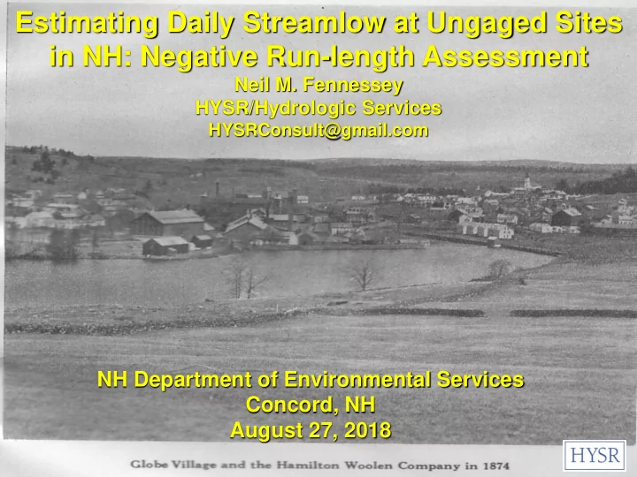
Estimating Daily Streamlow at Ungaged Sites in NH: Negative Run-length Assessment Neil M. Fennessey HYSR/Hydrologic Services HYSRConsult@gmail.com NH Department of Environmental Services Concord, NH August 27, 2018

Estimating Daily Flows at Ungaged Sites  NH DES needs to determine PIFs at ungaged sites in presently and future designated rivers  NHDES needs a reliable way to estimate daily streamflow time series at these ungaged sites  The QPPQ Transform method is one approach  Conceived and developed by Fennessey (1994)  Has been used in the northeast and central US, Canada and South Africa

Other Ways to Estimate Daily Flows at Ungaged Sites: Pluses & Minuses  Watershed Area Ratio (WAR) method  Very simple to use  Assumes that all watersheds are exactly alike except for the size of the watershed  Rainfall-Runoff Models (HSPF, Sacramento Soil Moisture Accounting Model)  Physically based but parameter-intensive  Used by NOAA for flood forecasting  Requires long stream gage period-of-record for site calibration and validation

Does USGS Like QPPQ Transform?  The QPPQ Transform method has been adopted or is being considered by several US Geological Survey district offices:  Massachusetts and Rhode Island USGS  Pennsylvania USGS  Iowa USGS  Minnesota USGS  New York USGS  New Hampshire and Vermont USGS

Has the QPPQ Been Extensively Tested?  The QPPQ Transform method was extensively tested by the USGS and bested 17 alternative methods for estimating daily flow time series at 182 gaged watershed sites located in  West Virginia  Tennessee  North Carolina  South Carolina  Georgia  Alabama  Florida

Have States or Agencies Adopted the QPPQ?  The QPPQ Transform method has been adopted by several state agencies:  Massachusetts EOEEA  Massachusetts DEP Water Management Act program  Sustainable Water Management Initiative  The Delaware River Basin Authority  Maryland Dept. of the Environment  Pennsylvania Dept. of Environmental Protection  New York State Energy R & D Authority  Minnesota Pollution Control Agency

Examples of Local Applications  The QPPQ Transform method has been used for  Many surface water reservoir system assessments in Massachusetts and Connecticut  River basin and watershed studies in Massachusetts and Connecticut  Systems analysis study of the Connecticut River watershed  Complex litigation in Connecticut

The QPPQ Transform Method

Four Steps to the QPPQ Transform Method 1. Chose a USGS Streamgage Site for the time series: Q gage (t) 2. Use that time series to construct a streamflow duration curve (FDC): Q gage (p) 3. Construct a FDC at the ungaged site using its watershed’s soil characteristics, climate, and topography and a regional FDC model: Q ungaged (p) 4. Generate a streamflow time series at the ungaged site: Q ungaged (t)

Minnesota USGS (Lorenz and Zigeweid, 2016)

Use Q gage (t) to Construct ‘observed’ FDC Q gage (p )  Rank sort Q gage (t) “n” days from largest to smallest Q (1) ≥ Q (2) ≥ Q (3) … Q (n-2) ≥ Q (n-1) ≥ Q (n)  “n” is number of days in the period of record  Use “plotting position” formula to estimate exceedance probability p=P[ Q≥q ]  “i” is the rank-order i=1,n POR 30 years x 365 = 10,950 days P[Q≥Q (n) ]x100 =10,950/10951 x 100 = 99.991

Step 1: Q gage (t) and Step 2: Q gage (p)  Common factor between the flow date, time, and the FDC probability, p, is Q = a 3-D relationship  Knowing Q gage (t) & p(Q gage ) => p(t)

Step 3: Regional FDC Model  Construct a FDC for the ungaged site without historic daily streamflow data

HYSR Phase 1 Study for NH DES: Update Regional FDC Model  Fennessey (2018) developed a special streamgage network of 133 USGS gaged watersheds in New England, NY, PA and NJ.  Daily streamflow data: minimum 20-year POR in 1950-1990 base period.  Research confirmed earlier Fennessey (1994) finding that the 3-parameter Generalize Pareto (GPA) was the best among alternatives.

 L-moments used to estimate the 3 GPA parameters: ζ , α , κ for each of 133 HYSR sites  Gather watershed specific data for each of these 133 USGS gage sites in the HYSR network  Use each of the 3 GPA parameters statistically determined for each HYSR watershed from obs streamgage data as dependent variables  Use OLS multivariate regression and each watershed’s specific soil, climate, and topography data as candidate independent variables  Keep only “statistically significant” soil, climate, and topographic variables to create one equation for each GPA parameter; ζ , α and κ .

 To construct a FDC at the ungaged site, the analyst must determine ten soil, climate, and topography characteristics for that watershed:  Watershed area (mi 2 )  Avg annual precipitation (in/yr)  Avg annual temperature ( o F)  Potential maximum soil moisture retention (in)  Percent of watershed area covered by HSG C soil (%)  Avg watershed elevation (ft)  Avg watershed aspect (degrees) 0-360 O  Percent of watershed area covered by lakes, ponds and reservoirs (%)  Percent of watershed area covered by impervious surface (%)  Slope of main stream channel (ft/mile)

Compare FDCs and Assess “Goodness-of-Fit” HYSR Phase 1 (Fennessey, 2018)  Construct “observed,” “fitted,” and regional “model” FDCs at eleven NH USGS gages sites, watershed areas range: 12.1 mi 2 – 622 mi 2  Graph all three FDCs for visual comparison  Estimate the Bias between the “observed” FDC and the “fitted” FDC to see how suitable the GPA is as basis for the Reginal FDC Model  Estimate the Bias between the “observed” FDC and the regional “model” FDC to see how well it compared with the “fitted” FDC.

Baker River, near Rumney, NH

QPPQ Transform Steps 1 - 3

 Assume for Steps 2 and 3: p(Q ungaged ) = p(Q gaged )

Step 4: Generate Q ungaged (t)  Recall 3-D relationship between t, Q and p => p(t)  Use regional FDC model with p(t) instead of just p

HYSR Phase 2 Study for NHDES Negative Run-length QPPQ Transform Assessment  In the Phase 2 study, HYSR focused on a negative run-length analysis of daily flows during bioperiods determined by fishery and other specialists at five USGS streamgage sites in New Hampshire  HYSR and NHDES reasoned that since Protected Instream Flow rates, PIFs, are determined in part by sub-threshold event durations, a negative run- length analysis would be a good way to further assess the QPPQ Transform method for use in New Hampshire

A Negative Run-length  A negative run-length event occurs when streamflow, Q(t), falls below a designated threshold, Q P , for one or more consecutive days.

Bioperiods  The University of New Hampshire et al (2007) study determined six PIF bioperiods for the Souhegan R. No. Bioperiod Start End 1 Over-Wintering 15-Nov 28-Feb 2 Spring Flood 1-Mar 30-Apr 3 Shad Spawning 1-May 14-Jun 4 GRAF Spawning 15-Jun 14-Jul 5 Rearing & Growth 15-Jul 30-Sep 6 Salmon Spawning 1-Oct 14-Nov

 The participants of the New Hampshire et al (2007) Souhegan River watershed study developed PIFs for each bioperiod  HYSR used two of these PIFs for the present study as negative run-length thresholds: Q critical and Q rare .  HYSR used Q 85 and Q 95 for the Diamond, Saco, Oyster and Pemigewasset Rivers because these watersheds do not yet have PIF flow rates.  Of particular interest to NHDES is the Rearing & Growth bioperiod which begins mid-summer and ends in early fall, when yearly flows are usually the lowest and the aquatic ecosystem quite stressed.

 During the 1963-1968 Rearing & Growth bioperiod, flows fell below Q critical (yellow) and Q rare (red) for long runs of time. 100 100 Q (cfs) 10 10 1 1 1964 1966 1968 Year

 During all Rearing & Growth days of flow over the entire POR, the FDC shows what fraction of time. Q critical ≈ Q 75,rearing & growth and Q rare ≈ Q 90,rearing & growth

 By counting the number of nday -long negative run- length events one constructs a frequency histogram for sub-Q critical events during Rearing & Growth.

 Similarly, one constructs a frequency histogram for sub-Q rare events that occurred over the POR during the 77 day-long Rearing & Growth bioperiod .

 If one wants to estimate the likelihood that a negative run-length of nday or more given that flows are sub-Q critical , one constructs a probability plot.

 Similarly, one may construct a probability plot for the negative run-length of nday or more given that flows are sub-Q rare . Called a Run Duration Curve (RDC)

Further QPPQ Transform Assessment  The QPPQ Transform is assessed by comparing negative run-length, season-specific FDCs, frequency histograms and probability plot RDCs.  Souhegan River assessment used Q critical and Q rare as event thresholds  Diamond, Saco, Oyster and Pemigewasset River assessments used Q 85 and Q 95 as event thresholds  Tests at these five sites were run using two different Index gages from the Fennessey (2018) 133 gage network as needed for Step 1 and 2 of the QPPQ Transform: HCDN NN and HCDN NN WA.