Estimates of Standard Model Backgrounds in Searches for New Physics - PowerPoint PPT Presentation

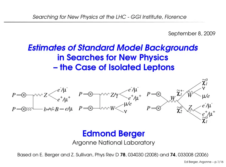
Searching for New Physics at the LHC - GGI Institute, Florence September 8, 2009 Estimates of Standard Model Backgrounds in Searches for New Physics – the Case of Isolated Leptons χ 0 1 ν e - / µ - e - / µ - χ +- P P Z/ γ P Z W 1 µ /e e + / µ + e + / µ + W µ /e e - / µ - Z e/ µ P W P χ 0 P B b ν e + / µ + 2 χ 0 1 Edmond Berger Argonne National Laboratory Based on E. Berger and Z. Sullivan, Phys Rev D 78 , 034030 (2008) and 74 , 033008 (2006) Ed Berger, Argonne – p.1/16

Outline 1. Several (1, 2, ... N) isolated leptons are a signature for New Physics 2. Many Standard Model sources of isolated leptons 3. New: Isolated leptons from heavy flavor ( b , c ) decays and cuts that can be used to deal with this background 4. Dileptons and the Search for Higgs Bosons: Summary Berger and Sullivan, Phys Rev D 74 , 033008 (2006) • H → WW → l + l − plus missing energy vs. leptons from Standard Model Sources at the LHC 5. Trileptons and the Search for Supersymmetry χ ± χ 0 • � 2 ( “Golden” SUSY channel) vs. leptons from 1 � Standard Model Sources at LHC 6. Conclusions Ed Berger, Argonne – p.2/16

Physics of isolated leptons from b decay Normalized Probability ✆ ✝ GeV � ☎ ✁ � ✂ ✄ ✞ ✆ ✝ GeV ☎ � ✁ ✂ ✄ 10 15 20 25 30 35 40 45 50 (GeV) ✟ ✠ ✞ Prob. isolated µ w. p T µ > 10 GeV = Prob. producing muon × Prob. B remnants missed • Muons that pass isolation take substantial fraction of p T b • Nearly all isolated muons point back to primary vertex. C. Wolfe, CDF internal • Isolation leaves ∼ 7 . 5 × 10 − 3 µ/b ≫ 10 − 4 per light jet Ed Berger, Argonne – p.3/16

Physics of isolated leptons from b decay 6 ✔ ✕ ✖ ✘ ✗ ✔ 5 ✕ ✖ ✘ ✗ Normalized Probability pb/GeV) ✧ ★ GeV ✦ ✜ ✢ ✣ ✥ ✤ 4 ✘ ✎ ✏ GeV ✙ ✡ ✍ ✚ ✛ ☛ ✡ ☞ ✌ ✑ ✲ ✱ 3 ✰ ( ✯ ✮ ✖ ✙ ✚ ✛ ✭ ✪ 2 ✬ ✫ ✪ 1 ✎ ✏ GeV ✍ ✡ ☛ ☞ ✌ 0 10 15 20 25 30 35 40 45 50 10 15 20 25 30 35 40 45 50 (GeV) (GeV) ✒ ✜ ✓ ✑ ✢ ✩ Fold in b ¯ Prob. isolated µ w. p T µ > 10 GeV b cross section • A large fraction of events with = Prob. producing muon × Prob. B remnants missed b → µ/e have isolated µ/e • Muons that pass isolation take • Long tail that extends to large substantial fraction of p T b momentum, but • Nearly all isolated muons point • 1 / 2 of all isolated µ come from back to primary vertex. b with p T b < 20 GeV . C. Wolfe, CDF internal It is common for analyses to start • Isolation leaves ∼ 7 . 5 × 10 − 3 µ/b simulations with p T b > 20 GeV ≫ 10 − 4 per light jet Ed Berger, Argonne – p.3/16

Dileptons at the LHC Higgs production and decay to WW Ed Berger, Argonne – p.4/16

ATLAS-like study; 160 GeV Higgs [ σ (fb)] b ¯ Wb ¯ bj ⋆ Cut level H → WW WW Wc single-top b Wc ¯ c Isolated l + l − > 10 GeV 336 1270 > 35700 12200 3010 1500 1110 E T l 1 > 20 GeV 324 1210 > 5650 11300 2550 1270 963 E T > 40 GeV / 244 661 > 3280 2710 726 364 468 M ll < 80 GeV 240 376 > 3270 2450 692 320 461 ∆ φ < 1 . 0 136 124 > 1670 609 115 94 131 | θ ll | < 0 . 9 81 83 > 1290 393 68 49 115 | η l 1 − η l 2 | < 1 . 5 76 71 > 678 320 48 24 104 Jet veto 41 43 > 557 175 11 12 7.4 130 < M ll T < 160 GeV 18 11 — 0.21 1.3 0.04 0.09 The biggest difference in the LHC analysis compared to our FNAL study is that cross sections are bigger, so the cuts are tighter. • After the / E T cut, all real power comes from the M ll T cut. Note S/B ∼ 1 at LHC, but let’s look at M ll T distribution Ed Berger, Argonne – p.5/16

Transverse mass distribution after cuts • Cannot reconstruct a Higgs boson mass peak from H → WW ∗ → l + l − ν ¯ ν ; use ‘transverse mass’ as an estimator; � M l ¯ 2 p l ¯ l T E miss l T = (1 − cos(∆ φ )) T ❑ ✹ ✹ ▲ ❖ ◗ ❇ ✽ ✳ ✳ ❙ ❚ ❋ ❙ ❯ ❏ ❈ ❈ ❉ ▼ ◆ ❉ ❆ ❈ ❆ ❘ ▼ ✺ ❍ P ✺ ❍ ❥ ❁ ✾ ❅ ✽ ✿ ❀ ❁ ❂ ❄ ❃ ✐ ❥ ✳ ✳ ✼ ✐ ❁ ❋ ■ ✹ ✹ ❏ ✳ ✴ ✵ ✳ ✵ ✹ ✴ ✴ ✵ ✶ ✶ ❆ ❃ ● ❍ ✸ ✷ ✸ ✺ ✻ ❇ ✹ ✹ ❊ ❆ ✸ ❈ ❈ ✺ ❉ ❢ ❸ ❷ ⑩ ❡ ❦ ❥ ⑨ ❼ ❞ ⑧ ❷ ❹ ❝ ⑦ ❦ ❁ ❼ ❜ ⑥ ❛ ⑤ ❷ ❺ ❵ ④ ❼ ❣ ❥ ❴ ③ ❪ ❫ ❷ ❻ ① ② ❪ ① ❭ ✇ ❼ ❣ ❁ ❷ ❶ ❨ t ❼ ❬ ✈ ❩ ✿ ❥ ✉ ❷ ❷ ❨ t ❼ ❺ ❷ ❹ ❷ ❸ ❷ ❷ ❸ ❶ ❷ ❸ ❻ ❷ ❸ ❺ ❷ ❸ ❹ ❷ ❶ ❷ ❷ ✿ ❁ ♠ ♠ ♦ ♣ s ❧ r q ♥ ❥ ❁ ❀ ❁ ❤ ❁ ✿ ❁ ❁ ✿ ❣ ❁ ✿ ✐ ❁ ✿ ❀ ❁ ✿ ❤ ❁ ❣ ❁ ❁ ❲ ❲ ✾ ❅ ❱ ❂ ❄ ❃ ❳ • Heavy flavor background is more than 10 times previous estimates of backgrounds when M l ¯ l T < 110 GeV; a tail extends into the signal region Ed Berger, Argonne – p.6/16

The transverse mass distribution at ATLAS 50 ❾ (160 GeV) 45 ❽ ❽ Heavy-flavor leptons 40 The HF background starts off 50 × the signal. min. ❿ ➀ ➁ 35 (fb/GeV) 1.0 T peak is ∼ 2 / 3 b ¯ The M ll bj ⋆ , ∼ 1 / 4 Wc ! 30 0.8 Wb ¯ 25 b , Wc ¯ c , single-top all are larger than WW . 0.6 ➉ ➊ ➉ ➈ 20 ➅ 0.4 ➇ The leading edge in M ll ➆ T covers m h = 140 GeV, 15 ➅ 0.2 10 0.0 and it bisects larger Higgs masses. 60 100 140 180 5 0 60 80 100 120 140 160 180 200 ➃ ➃ ➂ (GeV) ➄ 1.0 ➋ (140 GeV) ➋ (160 GeV) ➋ (180 GeV) 0.8 min. HF leptons ➋ (200 GeV) (fb/GeV) 0.6 ➓ ➔ ➓ ➒ 0.4 ➏ ➑ ➐ ➏ 0.2 0.0 60 80 100 120 140 160 180 200 ➍ ➍ ➌ (GeV) ➎ Ed Berger, Argonne – p.7/16

The transverse mass distribution at ATLAS 50 ➣ (160 GeV) 45 → → Heavy-flavor leptons 40 The HF background starts off 50 × the signal. min. ↔ ↕ ➙ 35 (fb/GeV) 1.0 T peak is ∼ 2 / 3 b ¯ The M ll bj ⋆ , ∼ 1 / 4 Wc ! 30 0.8 Wb ¯ 25 b , Wc ¯ c , single-top all are larger than WW . 0.6 ➢ ➤ ➢ ➡ 20 ➞ 0.4 ➠ The leading edge in M ll ➟ T covers m h = 140 GeV, 15 ➞ 0.2 10 0.0 and it bisects larger Higgs masses. 60 100 140 180 5 ATLAS proposes a very tight cut: 0 60 80 100 120 140 160 180 200 ➜ ➜ m h − 30(40) GeV < M ll ➛ (GeV) T < m h ➝ 1.0 and attempts to extract the upper shoulder of ➥ (140 GeV) ➥ (160 GeV) ➥ (180 GeV) 0.8 H → WW from the upper shoulder of WW . min. HF leptons ➥ (200 GeV) (fb/GeV) / cut m h / 2 < M ll D 0 T < m h − 10 GeV — goes for peak. 0.6 ➲ ➳ Since the shapes for m h � > 160 GeV are so similar, ➲ ➯ 0.4 ➩ ➭ ➫ everything relies on counting events in the tails. ➩ 0.2 0.0 60 80 100 120 140 160 180 200 ➧ ➧ ➦ (GeV) ➨ Ed Berger, Argonne – p.7/16

The transverse mass distribution at ATLAS 50 ➸ (160 GeV) 45 ➵ ➵ Heavy-flavor leptons 40 The HF background starts off 50 × the signal. min. ➺ ➻ ➼ 35 (fb/GeV) 1.0 T peak is ∼ 2 / 3 b ¯ The M ll bj ⋆ , ∼ 1 / 4 Wc ! 30 0.8 Wb ¯ 25 b , Wc ¯ c , single-top all are larger than WW . 0.6 ➴ ➷ ➴ ➘ 20 ➪ 0.4 ➹ The leading edge in M ll ➶ T covers m h = 140 GeV, 15 ➪ 0.2 10 0.0 and it bisects larger Higgs masses. 60 100 140 180 5 ATLAS proposes a very tight cut: 0 60 80 100 120 140 160 180 200 ➾ ➾ m h − 30(40) GeV < M ll ➽ (GeV) T < m h ➚ 1.0 and attempts to extract the upper shoulder of ➬ (140 GeV) ➬ (160 GeV) ➬ (180 GeV) 0.8 H → WW from the upper shoulder of WW . min. HF leptons ➬ (200 GeV) (fb/GeV) / cut m h / 2 < M ll D 0 T < m h − 10 GeV — goes for peak. 0.6 Ï Ð Since the shapes for m h � > 160 GeV are so similar, Ï ❰ 0.4 ❐ ❮ ❒ everything relies on counting events in the tails. ❐ 0.2 If WW were the only background, this might work. 0.0 60 80 100 120 140 160 180 200 ➱ ➱ ➮ (GeV) ✃ Cannot predict to 10–20 GeV the position of HF leading edge. However, can measure the HF background . . . and maybe cut it. Ed Berger, Argonne – p.7/16

One very effective new cut . . . Most variations of cuts do not help much. One could try to raise the cut on p T l 1 . Õ Ó Ó Ö Ó • No help vs. anything with a W . ä Ô â ã Single top Ò Ñ Ñ min. (fb/GeV) • Even b ¯ b does not decrease fast enough. å â ã Recall, an “isolated lepton” from a B is usually á à ß Þ not soft compared to the B . Û Ý Ü æ Û â ã However, the second lepton p T falls exponentially. So raise the cut: p T l 2 > 10 GeV ⇒ p T l 2 > 20 GeV. ç â ã 20 25 30 35 40 45 50 55 60 65 70 × (GeV) Ø Ù Ú ì ê ê í ê û ë ù ú Single top é min. è è (fb/GeV) ü ù ú ø ÷ ö õ ò ô ó ò ý ù ú þ ù ú 10 15 20 25 30 35 40 45 50 î (GeV) ï ð ñ Ed Berger, Argonne – p.8/16