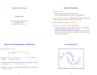
kernel CCA, kernel Kmeans Spectral Clustering 1 MACHINE LEARNING - PowerPoint PPT Presentation

MACHINE LEARNING – 2012 Applications of Kernel CCA Goal: To measure correlation between heterogeneous datasets and to extract sets of genes which share similarities with respect to multiple biological attributes Kernel matrices K1, K2 and K3 correspond to gene-gene similarities in pathways, genome position, and microarray expression data resp. Correlation scores in MKCCA: Use RBF kernel with fixed kernel width. pathway vs. genome vs. expression. Y Yamanishi, JP Vert, A Nakaya, M Kanehisa - Extraction of correlated gene clusters from multiple genomic data by generalized kernel canonical correlation analysis, Bioinformatics, 2003 21

MACHINE LEARNING – 2012 Applications of Kernel CCA Goal: To measure correlation between heterogeneous datasets and to extract sets of genes which share similarities with respect to multiple biological attributes Gives pairwise correlation between K1, K2 Gives pairwise correlation between K1, K3 Two clusters correspond to genes close to each other with respect to their positions in the pathways, in the genome, and to their expression A readout of the entries with equal projection onto the first canonical vectors  give the genes which Correlation scores in MKCCA: belong to each cluster pathway vs. genome vs. expression. Y Yamanishi, JP Vert, A Nakaya, M Kanehisa - Extraction of correlated gene clusters from multiple genomic data by generalized kernel canonical correlation analysis, Bioinformatics, 2003 22

MACHINE LEARNING – 2012 Applications of Kernel CCA Goal: To construct appearance models for estimating an object’s pose from raw brightness images X: Set of images Y: pose parameters (pan and tilt angle of the object w.r.t. the camera in degrees) Example of two image datapoints with different poses Use linear kernel on X and RBF kernel on Y and compare performance to applying PCA on the (X, Y) dataset directly T. Melzer, M. Reiter and H. Bischof, Appearance models based on kernel canonical correlation analysis, Pattern Recognition 36 (2003) p. 1961 – 1971 23

MACHINE LEARNING – 2012 Applications of Kernel CCA Goal: To construct appearance models for estimating an object’s pose from raw brightness images kernel-CCA performs better than PCA, especially for small k=testing/training ratio (i.e., for larger training sets). The kernel-CCA estimators tend to produce less outliers, i.e., gross errors, and consequently yield a smaller standard deviation of the pose estimation error than their PCA-based counterparts. Testing/training ratio For very small training sets, the performance of both approaches becomes similar T. Melzer, M. Reiter and H. Bischof, Appearance models based on kernel canonical correlation analysis, Pattern Recognition 36 (2003) p. 1961 – 1971 24

MACHINE LEARNING – 2012 Kernel K-means Spectral Clustering 26

MACHINE LEARNING – 2012 Structure Discovery: Clustering Groups pair of points according to how similar these are. Density based clustering methods (Soft K-means, Kernel K-means, Gaussian Mixture Models) compare the relative distributions. 27

MACHINE LEARNING – 2012 K-means K-means is a hard partitioning of the space through K clusters equidistant according to norm 2 measure. The distribution of data within each cluster is encapsulated in a sphere. * m 2 * m1 * m 3 28

MACHINE LEARNING – 2012 K-means Algorithm k k m  , 1... , K 29

MACHINE LEARNING – 2012 K-means Algorithm Iterative Method (variant on Expectation-Maximization) 2. Calculate the distance from each data point to each centroid .   p m   m j k j k , d x x 3. Assignment Step: Assign the responsibility of each data point to its “closest” centroid ( E-step). If a tie happens (i.e. two centroids are equidistant to a data     point, one assigns the data point to the smallest winning centroid). m argmin , d x j k k 30

MACHINE LEARNING – 2012 K-means Algorithm Iterative Method (variant on Expectation-Maximization) 2. Calculate the distance from each data point to each centroid .   p m   m j k j k , d x x 3. Assignment Step: Assign the responsibility of each data point to its “closest” centroid ( E-step). If a tie happens (i.e. two centroids are equidistant to a data     point, one assigns the data point to the smallest winning centroid). m argmin , d x j k k Update Step: Adjust the centroids to be the means of all data points 4. assigned to them (M-step) 5. Go back to step 2 and repeat the process until the clusters are stable. 31

MACHINE LEARNING – 2012 K-means Clustering: Weaknesses Two hyperparameters : number of clusters K and power p of the metric Very sensitive to the choice of the number of clusters K and the initialization. 32

MACHINE LEARNING – 2012 K-means Clustering: Hyperparameters Two hyperparameters : number of clusters K and power p of the metric Choice of power determines the form of the decision boundaries P=2 P=1 P=3 P=4 33

MACHINE LEARNING – 2012 Kernel K-means K-Means algorithm consists of minimization of:   j x   K   p m m   m m  1 j k K j k k ,...., with x C J x m   j k 1 k x C k k : number of datapoints in cluster m C k   1 Project into a feature space   M f x i  i p       K   m m  f  f m 1 K j k ,...., J x     j k 1  k x C f j x  j k x C m k We cannot observe the mean in feature space.  Construct the mean in feature space using image of points in same cluster 34

MACHINE LEARNING – 2012 Kernel K-means 2       K   m m  f  f m 1 K j k ,...., J x  j  k 1 k x C             f f f f j l l j 2 x x x x       K   f f   j l  k  l k , j j x x C x C =  x x    2 m m    j  k k 1 x C k k           j l i j k , x x 2 k , x x     K       j l k j k i i x , x C = k , x C  x x    2 m m     j k 1 k x C k k   35

MACHINE LEARNING – 2012 Kernel K-means Kernel K-means algorithm is also an iterative procedure: 1. Initialization: pick K clusters 2. Assignment Step: Assign each data point to its “closest” centroid ( E-step). If a tie happens (i.e. two centroids are equidistant to a data point, one assigns the data point to the smallest winning centroid) by computing the distance in feature space.         j l i j k , x x 2 k , x x           j l k  j k , i k i i x x C x C min , min k ,   d x C x x   2 m k k m   k k   3. Update Step: Update the list of points belonging to each centroid (M-step) 4. Go back to step 2 and repeat the process until the clusters are stable. 36

MACHINE LEARNING – 2012 Kernel K-means With a RBF kernel If the points are well grouped in If xi is close to all points cluster k, this sum in cluster k, this is close is close to 1. to 1. Cst of value 1         j l i j k , x x 2 k , x x           j l k  j k , i k i i x x C x C min , min k ,   d x C x x   2 m k k m   k k   With homogeneous polynomial kernel? 37

MACHINE LEARNING – 2012 Kernel K-means With a polynomial kernel Some of the terms If the points are change sign depending aligned in the on their position with same Quadran, respect to the origin. the sum is Positive value maximal         j l i j k , x x 2 k , x x           j l k  j k , i k i i x x C x C min , min k ,   d x C x x   2 m k k m   k k   38

MACHINE LEARNING – 2012 Kernel K-means: examples Rbf Kernel, 2 Clusters 39

MACHINE LEARNING – 2012 Kernel K-means: examples Rbf Kernel, 2 Clusters 40

MACHINE LEARNING – 2012 Kernel K-means: examples Rbf Kernel, 2 Clusters Kernel width: 0.5 Kernel width: 0.05 41

MACHINE LEARNING – 2012 Kernel K-means: examples Polynomial Kernel, 2 Clusters 42

MACHINE LEARNING – 2012 Kernel K-means: examples Polynomial Kernel (p=8), 2 Clusters 43

MACHINE LEARNING – 2012 Kernel K-means: examples Polynomial Kernel, 2 Clusters Order 2 Order 4 Order 6 44

MACHINE LEARNING – 2012 Kernel K-means: examples Polynomial Kernel, 2 Clusters The separating line will always be perpendicular to the line passing by the origin (which is located at the mean of the datapoints) and parrallel to the axis of the ordinates (because of the change in sign of the cosine function in the inner product.  No better than linear K-means! 45

MACHINE LEARNING – 2012 Kernel K-means: examples Polynomial Kernel, 4 Clusters Solutions found with Kernel K-means Solutions found with K-means Can only group datapoints that do not overlap across quadrans with respect to the origin (careful, data are centered!).  No better than linear K-means! (except less sensitive to random initialization) 46

MACHINE LEARNING – 2012 Kernel K-means: Limitations Choice of number of Clusters in Kernel K-means is important 47

MACHINE LEARNING – 2012 Kernel K-means: Limitations Choice of number of Clusters in Kernel K-means is important 48

MACHINE LEARNING – 2012 Kernel K-means: Limitations Choice of number of Clusters in Kernel K-means is important 49

MACHINE LEARNING – 2012 Limitations of kernel K-means Raw Data 50

MACHINE LEARNING – 2012 Limitations of kernel K-means kernel K-means with K=3, RBF kernel 51

MACHINE LEARNING – 2012 From Non-Linear Manifolds Laplacian Eigenmaps, Isomaps To Spectral Clustering 52

MACHINE LEARNING – 2012 Non-Linear Manifolds PCA and Kernel PCA belong to a more general class of methods to create non-linear manifolds based on spectral decomposition . (Spectral decomposition of matrices is more frequently referred to as an eigenvalue decomposition.) Depending on which matrix we decompose, we get a different set of projections. • PCA decomposes the covariance matrix of the dataset  generate rotation and projection in the original space • kernel PCA decomposes the Gram matrix  partition or regroup the datapoints • The Laplacian matrix is a matrix representation of a graph. Its spectral decomposition can be used for clustering. 53

MACHINE LEARNING – 2012 Embed Data in a Graph Original dataset Graph representation of the dataset • Build a similarity graph • Each vertex on the graph is a datapoint 54

MACHINE LEARNING – 2012 Measure Distances in Graph   0.9.....0.8. .. 0.2 ... 0.2     ..... S     0.2.....0.2........0.7....0.6  Construct the similarity matrix S to denote whether points are close or far away to weight the edges of the graph: 55

MACHINE LEARNING – 2012 Disconnected Graphs   1.........1. .. .....0 .......0     ..... S  Disconnected Graph:   Two data-points are connected if:  0.........0..........1.........1  a) the similarity between them is higher than a threshold. b) or if they are k-nearest neighbors (according to the similarity metric) 56

MACHINE LEARNING – 2012 Graph Laplacian   1.........1. .. .....0 .......0     Given the similarity matrix ..... S    0.........0..........1.........1   Construct the diagonal matrix D composed of the sum on each line of K:    ............. ...0 S 1 i   i    0 ........0 S   2 i  , D   i   ....    0.................. S   Mi   i   and then, build the Laplacian matrix : L D S  L is positive semi-definite spectral decomposition possible 57

MACHINE LEARNING – 2012 Graph Laplacian Eigenvalue decomposition of the Laplacian matrix:   T L U U All eigenvalues of L are positive and the smallest eigenvalue of L is zero:  If we order the eigenvalue by increasing order:        0 .... . 1 2 M If the graph has connected components, then the k  eigenvalue =0 has multiplicity . k 58

MACHINE LEARNING – 2012 Spectral Clustering  The multiplicity of the eigenvalue 0 determines the number of connected components in a graph. The associated eigenvectors identify these connected components.   i For an eigenvalue 0, the correspondin g eigenvector has the same value e i  for all vertices in a component,and a different value for each one of their i 1 components. Identifying the clusters is then trivial when the similarity matrix is composed of zeros and ones (as when using k-nearest neighbor). What happens when the similarity matrix is full? 59

MACHINE LEARNING – 2012 Spectral Clustering   0.9.....0.8. .. 0.2 ... 0.2       N N Similarity map : S ..... S    can either be binary (k-nearest neighboor) S  0.2.....0.2........0.7....0.6  or continuous with Gaussia kernel  i j x x      2 i j , 2 S x x e 60

MACHINE LEARNING – 2012 Spectral Clustering   1) Build the Laplacian matrix : L D S   T 2) Do eigenvalue decomposition of the Laplacian matrix: L U U 3) Order the eigenvalue by increasing order:        0 .... . 1 2 M The first eigenvalue is still zero but with multiplicity 1 only (fully connected graph)! Idea: the smallest eigenvalues are close to zero and hence provide also information on the partioning of the graph (see exercise session)   N N Similarity map : S can either be binary (k-nearest neighboor) S or continuous with Gaussia kernel  i j x x      2 i j , 2 S x x e 61

MACHINE LEARNING – 2012 Spectral Clustering Eigenvalue decomposition of the Laplacian matrix:   T L U U Construct an embedding of each of the   1 2 K   ........ 1 e e e i i e M datapoints through . x y 1 1 1   i   1 Reduce dimensionality by picking k<M   . e   2       i i . projections , 1... . . y i K y      U   . .       K .   e   i   1 2 K  ........  e e e 1 1 M With a clear partitioning of the graph, the entries in y are split into sets of equal values. Each group of points with same value belong to the same partition (cluster). 62

MACHINE LEARNING – 2012 Spectral Clustering Eigenvalue decomposition of the Laplacian matrix:   T L U U Construct an embedding of each of the   1 2 K   ........ 1 e e e i i e M datapoints through . x y 1 1 1   i   1   Reduce dimensionality by picking k<M . e   2       i i . projections , 1... . . y i K y      U   .   .     K .   e   i   1 2 K  ........  e e e M 1 1 When we have a fully connected graph, the entries in Y take any real value. 63

MACHINE LEARNING – 2012 Spectral Clustering Example: 3 datapoints in a graph composed of 2 partitions   1 1 0 1 x     The similarity matrix is 1 1 0 S  2 x    0 0 1  3  x has eigenvalue =0 with multiplicity two. L One solution for the two associated eigenvectors is:   Anothersolution for the two associated eigenvectors is: 1    1   2 1 e 0.33   Entries in the       1   0 0.33 eigenvector for the e  two first datapoins       0.88  0 are equal      2    0 e 0.1       1 1 1 0 0.33 -0.1 y y         1 2 0.1 e         2 2 1 0 0.33 -0.1 y y    0.99  for the 1st set of eigenvectors for the 2nd set of eigenvectors 64

MACHINE LEARNING – 2012 Spectral Clustering Example: 3 datapoints in a fully connected graph   1 0.9 0.02   1 x   The similarity matrix is 0.9 1 0.02 S    2  0.01 0.02 1  x  has eigenvalue =0 with multiplicity 1. The seco nd L 3 x   eigenvalue is small 0.04, whereas the 3rd one 2   is large, 1.81. Entries in the 2 nd 3 eigenvector for the with associated eigenvectors : two first datapoins are almost equal.        1 0.411 0.8          1 2 3 2 1 , 0.404 , 0.7 e e e             1 2        1 0.41 , 1 0.40 y y   1  0.81   0.0  The first two points have almost the same coordinates on the y embedding. Reduce the dimensionality by considering the smallest eigenvalue 65

MACHINE LEARNING – 2012 The 3 rd point is now Spectral Clustering closer to the two other points Example: 3 datapoints in a fully connected graph   1 0.9 0.8 1 x     The similarity matrix is 0.9 1 0.7 S  2   x  0.8 0.7 1  3 x  has eigenvalue =0 with multiplicity 1. The secon d L     and third eigenvalues are both large 2.23, 2.57. 2 3 Entries in the 2 nd eigenvector for the two first datapoins are with associated eigenvectors : no longer equal.         1 0.21 0.78           1 2 3 2 1 , 0.57 , 0.57 e e e                   1 2   1  0.79   0.21  1 -0.21 , 1 -0.57 y y The first two points have no longer the same coordinates on the y embedding. 66

MACHINE LEARNING – 2012 Spectral Clustering 2 x w 1 y 1 12 x 2 y 3 y 3 x w 21 6 y 6 x 4 y 4 x Step 1: Embedding in y 5 y 5 x Idea: Points close to one another have almost the same coordinate on the eigenvectors of L with small eigenvalues. Step1: Do an eigenvalue decomposition of the Lagrange matrix L and project the datapoints onto the first K eigenvectors with smallest eigenvalue (hence reducing the dimensionality). 67

MACHINE LEARNING – 2012 Spectral Clustering 2 x w 1 y 1 12 x 2 y 3 y 3 x w 21 6 y 6 x 4 y 4 x 5 y 5 x Step 2: 1 M Perform K-Means on the set of ,... vectors y y Cluster datapoints x according to their clustering in y. 68

MACHINE LEARNING – 2012 Equivalency to other non-linear Embeddings Spectral deomposition of the similarity matrix (which is already positive semi-definite)    1 e  1 i  In Isomap, the embedding is   . normalized by the eigenvalues      i . y  and uses geodesic distance to build   . the similarity matrix,    K see supplementary material. e   K i 70

MACHINE LEARNING – 2012 Laplacian Eigenmaps   Solve the generalized eigenvalue problem: Ly Dy  T T Solution to optimization problem: min such that 1. y Ly y Dy y Ensures minimal distorsion while preventing arbitrary scaling. Swissroll example Projections on each Laplacian eigenvector  i The vectors , 1... , form an embedding of the datapoints. y i M Image courtesy from A. Singh 71

MACHINE LEARNING – 2012 Equivalency to other non-linear Embeddings kernel PCA: Eigenvalue decomposition of the matrix of similarity S  T S UDU The choice of parameters in kernel K-Means can be initialized by doing a readout of the Gram matrix after kernel PCA. 72

MACHINE LEARNING – 2012 Kernel K-means and Kernel PCA The optimization problem of kernel K-means is equivalent to: 1 See paper by M. Welling,    T max , 2 tr H KH H YD   supplementary document on website H M   Look at the eigenvalues to determine     T Since , tr H KH  optimal number of clusters. i  1 i  : M eigenvalues, resulting from the eigenvalue decomposition i of the Gram Matrix  : Y M K Each entry of Y is 1 if the datapoint belongs to cluster k, otherwise zero  : D is diagonal. Element on the diagonal is sum of the datapoint in cluster k D K K 73

MACHINE LEARNING – 2012 Kernel PCA projections can also help determine the kernel width From top to bottom Kernel width of 0.8, 1.5, 2.5 74

MACHINE LEARNING – 2012 Kernel PCA projections can help determine the kernel width The sum of eigenvalue grows as we get a better clustering 75

MACHINE LEARNING – 2012 Quick Recap of Gaussian Mixture Model 76

MACHINE LEARNING – 2012 Clustering with Mixture of Gaussians Alternative to K-means; soft partitioning with elliptic clusters instead of spheres Clustering with Mixtures of Gaussians using spherical Gaussians (left) and non spherical Gaussians (i.e. with full covariance matrix) (right). Notice how the clusters become elongated along the direction of the clusters (the grey circles represent the first and second variances of the distributions). 77

MACHINE LEARNING – 2012 Gaussian Mixture Model (GMM)    1,... i M  Using a set of M N- dimensional training datapoints i X x j  1,... j N The pdf of X will be modeled through a mixture of K Gaussians:       K       m  m   m  i i i i i i | , , with | , , p X p X p X N i  i 1 m  i i , : mean and covariance matrix of Gaussian i K    1 Mixing Coefficients i  1 i   M       j | p i p i x Probability that the data was explained by i Gaussian i:  1 j 78

MACHINE LEARNING – 2012 Gaussian Mixture Modeling The parameters of a GMM are the means, covariance matrices and prior pdf :     m m     1 1 1 K K K ,..... , ,..... , ,..... Estimation of all the parameters can be done through Expectation- Maximization (E-M). E-M tries to find the optimum of the likelihood of the model given the data, i.e.:        max | max | L X p X   See lecture notes for details 79

MACHINE LEARNING – 2012 Gaussian Mixture Model 80

MACHINE LEARNING – 2012 Gaussian Mixture Model GMM using 4 Gaussians with random initialization 81

MACHINE LEARNING – 2012 Gaussian Mixture Model Expectation Maximization is very sensitive to initial conditions: GMM using 4 Gaussians with new random initialization 82

MACHINE LEARNING – 2012 Gaussian Mixture Model Very sensitive to choice of number of Gaussians. Number of Gaussians can be optimized iteratively using AIC or BIC, like for K-means: Here, GMM using 8 Gaussians 83

MACHINE LEARNING – 2012 Evaluation of Clustering Methods 84

MACHINE LEARNING – 2012 Evaluation of Clustering Methods Clustering methods rely on hyper parameters • Number of clusters • Kernel parameters  Need to determine the goodness of these choices Clustering is unsupervised classification  Do not know the real number of clusters and the data labels  Difficult to evaluate these choice without ground truth 85

MACHINE LEARNING – 2012 Evaluation of Clustering Methods Two types of measures: Internal versus external measures Internal measures rely on measure of similarity (e.g. intra-cluster distance versus inter-cluster distances) E.g.: Residual Sum of Square is an internal measure (available in mldemos); Gives the squared distance of each vector from its centroid summed over all vectors. K  2  m k RSS= x   1 k x C k  Internal measures are problematic as the metric of similarity is often already optimized by clustering algorithm 86

MACHINE LEARNING – 2012 Evaluation of Clustering Methods K-Means, soft-K-Means and GMM have several hyperparameters: (Fixed number of clusters, beta, number of Gaussian functions)  Measure to determine how well the choice of hyperparameters fit the dataset (maximum-likelihood measure) : dataset; : number of datapoints; : number of free parameters X M B   - Aikaike Information Criterion: AIC= 2ln 2 L B Penalty for      increase in - Bayesian Information Criterion: 2ln ln BIC L B M computational L: maximum likelihood of the model giv en B parameters costs Choosing AIC versus BIC depends on the application: Lower BIC implies either fewer explanatory variables, better fit, or both.  Is the purpose of the analysis to make predictions, or to decide which model As the number of datapoints (observations) increase, BIC assigns more weights best represents reality? AIC may have better predictive ability than BIC, but BIC finds a computationally to simpler models than AIC. more efficient solution. 87

MACHINE LEARNING – 2012 Evaluation of Clustering Methods Two types of measures: Internal versus external measures External measures assume that a subset of datapoints have class label and measures how well these datapoints are clustered.  Needs to have an idea of the class and have labeled some datapoints  Interesting only in cases when labeling is highly time-consuming when the data is very large (e.g. in speech recognition) 88

MACHINE LEARNING – 2012 Evaluation of Clustering Methods Raw Data 89

MACHINE LEARNING – 2012 Semi-Supervised Learning Clustering F-Measure: (careful: similar but not the same F-measure as the F-measure we will see for classification!) Tradeoff between clustering correctly all datapoints of the same class in the same cluster and making sure that each cluster contains points of only one class.    : nm of datapoints, : the set of classes M C c i Picks for each class : nm of clusters, K the cluster with the : nm of members of class and of cluster n c k ik i maximal number of c         i datapoints , max , F C K F c k i M  c C k i     2 , , Recall : proportion of R c k P c k    i i , F c k      i datapoints correctly , , R c k P c k i i classified/clusterized n    ik , R c k i c Precision : proportion of i n   datapoints of the same  ik , P c k i k class in the cluster 90

MACHINE LEARNING – 2012 Evaluation of Clustering Methods RSS with K-means can find the true optimal number of clusters but very sensitive to random initialization (left and right: two different runs). RSS finds an optimum for K=4 and K=5 for the right run 91

MACHINE LEARNING – 2012 Evaluation of Clustering Methods BIC (left) and AIC (right) perform very poorly here, splitting some clusters into two halves. 92

MACHINE LEARNING – 2012 Evaluation of Clustering Methods BIC (left) and AIC (right) perform much better for picking the right number of clusters in GMM. 93

MACHINE LEARNING – 2012 Evaluation of Clustering Methods Raw Data 94

MACHINE LEARNING – 2012 Evaluation of Clustering Methods Optimization with BIC using K-means 95

MACHINE LEARNING – 2012 Evaluation of Clustering Methods Optimization with AIC using K-means AIC tends to find more clusters 96

MACHINE LEARNING – 2012 Evaluation of Clustering Methods Raw Data 97

MACHINE LEARNING – 2012 Evaluation of Clustering Methods Optimization with AIC using kernel K-means with RBF 98

MACHINE LEARNING – 2012 Evaluation of Clustering Methods Optimization with BIC using kernel K-means with RBF 99

MACHINE LEARNING – 2012 Semi-Supervised Learning Raw Data: 3 classes 100

MACHINE LEARNING – 2012 Semi-Supervised Learning Clustering with RBF kernel K-Means after optimization with BIC 101

MACHINE LEARNING – 2012 Semi-Supervised Learning After semi-supervised learning 102