ENERGY-EFFICIENT COOPERATIVE ADAPTIVE CRUISE CONTROL OF PLATOONING - PowerPoint PPT Presentation

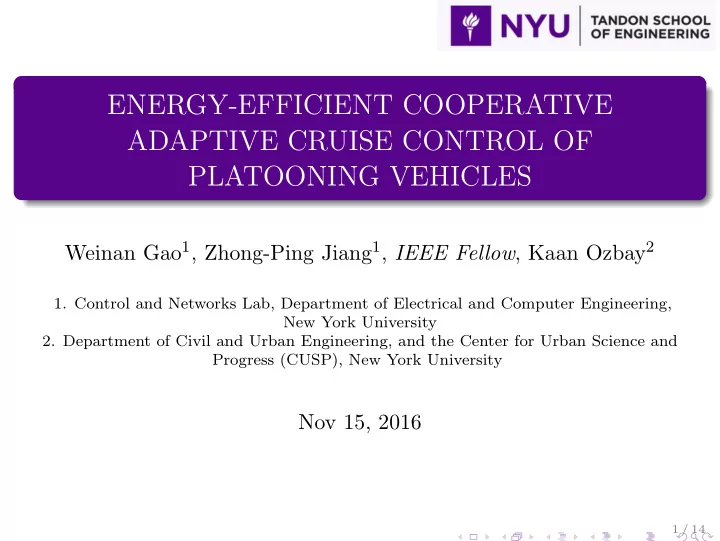
ENERGY-EFFICIENT COOPERATIVE ADAPTIVE CRUISE CONTROL OF PLATOONING VEHICLES Weinan Gao 1 , Zhong-Ping Jiang 1 , IEEE Fellow , Kaan Ozbay 2 1. Control and Networks Lab, Department of Electrical and Computer Engineering, New York University 2. Department of Civil and Urban Engineering, and the Center for Urban Science and Progress (CUSP), New York University Nov 15, 2016 1 / 14

Background and Motivation It’s imperative to develop next-generation Background: cruise controllers for connected vehicles to increase the safety, reliability, connectivity There are over 1 million road traffic and autonomy. deaths worldwide every year. [Challenge]: 90% of accidents are attributed to human errors Parametric variations → Unknown 1 system parameters Americans were stuck in traffic for 8 billion hours in 2015. Uncertain models of to-be-followed 2 vehicles ”We are the first generation that can end poverty, the last that can end Energy efficient → Eco-friendly 3 climate change.” – Ban Ki-Moon. Input(acceleration) saturation 4 2 / 14

Background and Motivation Adaptive control approaches for 1 platooning vehicles are not optimal [Swaroop, Hedrick & Choi 2001], [Kwon & Chua 2014]. Optimal control methods are usually 2 model-based and not data-driven. [Jovanovic & Bamieh 2005], [Waschl, Kolmanovsky, Steinbuch, & del Re 2014]. Reinforcement-learning-based controllers 3 cannot guarantee the stability of the closed-loop systems [Ng et al. 2008], [Desjardins & Chaib-draa 2011] We develop a data-driven, non-model-based adaptive optimal controller for platooning vehicles by Adaptive Dynamics Programming (ADP). The issue of input saturation is also addressed. 1Gao, W.; Jiang, Z. P. & Ozbay, K. Data-driven Adaptive optimal control of connected vehicles, IEEE Transactions on Intelligent Transportation Systems , 2016. 3 / 14

Background and Motivation Dynamic Programming [Bellman 1957] 1 Curse of dimensionality 2 Curse of modeling [Werbos 1968] pointed out that adaptive approximation to the HJB equation can be achieved by designing appropriate learning systems: approximate/adaptive dynamic programming (ADP) 1 Heuristic dynamic programming: approximate the optimal cost function. 2 Dual dynamic programming: approximate the gradient of the optimal cost function. 4 / 14

Review on ADP and Adaptive Optimal Control The platoon can be modeled by the following systems x = Ax + Bu ˙ � ∞ x T ( τ ) Qx ( τ ) + u T ( τ ) Ru ( τ ) J ( x 0 ) = � � dτ 0 The optimal control policy u = − R − 1 B T P ∗ x := − K ∗ x where P ∗ = P ∗ T > 0 is the unique solution to Riccati equation A T P ∗ + P ∗ A + Q − P ∗ BR − 1 B T P ∗ = 0 Adaptive optimal control: find P ∗ and K ∗ when A and B are unknown 5 / 14

Review on ADP and Adaptive Optimal Control [Jiang & Jiang 2012] Adaptive optimal control with unknown system matrices A and B 1 Start from an admissible K 0 . k ← 0. � t 1 2 x T ( t 1 ) P k x ( t 1 ) − x ( t 0 ) T P k x ( t 0 ) = − t 0 x T ( Q + K T k RK k ) xdτ + � t 1 t 0 ( u + K k x ) T RK k +1 xdτ 2 3 k ← k + 1. Repeat Step 2. k →∞ P k = P ∗ and lim Both can ensure lim k →∞ K k = K ∗ . 2Jiang, Y. & Jiang, Z. P. Computational adaptive optimal control for continuous-time linear systems with completely unknown dynamics, Automatica , 2012, 48, 2699-2704. 6 / 14

Paramics Micro-Traffic Simulation Results Double-loop ADP algorithm Traffic simulation architecture 1Gao, W.; Jiang, Z. P. & Ozbay, K. Data-driven Adaptive optimal control of connected vehicles, IEEE Transactions on Intelligent Transportation Systems , 2016. 7 / 14

Paramics Micro-Traffic Simulation Results ( a ) ( b ) 4000 6000 ( a ) 25 3500 h 2 h 3 5000 20 h 4 h i [ m ] 3000 h 5 15 4000 2500 10 0 5 10 15 20 25 30 2000 3000 t [ s ] ( b ) 20 1500 2000 v 1 v 2 1000 15 v 3 v i [ m/s ] v 4 1000 v 5 500 10 0 0 5 −10 −5 0 5 10 −10 −5 0 5 10 0 5 10 15 20 25 30 Acceleration [ m/s 2 ] Acceleration [ m/s 2 ] t [ s ] Histograms of accelerations Plots of headways and velocities 8 / 14

Paramics Micro-Traffic Simulation Result 9 / 14

Nonlinear and Adaptive Optimal Control of Platooning Vehicles Employ global ADP (GADP)[Jiang and Jiang 2015] to solve a longstanding issue in ITS: how to take into account strong nonlinearity and unknown dynamics in the design of global adaptive optimal controllers. Contributions: Because of the strongly nonlinear dynamics of the platooning vehicles, we are not aware of any global solutions to adaptive optimal control of platooning vehicles with unknown dynamics. Different from existing adaptive control approaches of platooning vehicles [Swaroop, Hedrick & Choi 2001], [Kwon & Chua 2014] the online GADP approach learns a near-optimal controller iteratively via real-time state/input data. The neural network approximation is avoided for this kind of high-order platooning vehicle systems which dramatically decreases the computational burden. 3Gao, W. & Jiang, Z. P., Nonlinear and Adaptive Suboptimal Control of Connected Vehicles: A Global Adaptive Dynamic Programming Approach. Journal of Intelligent & Robotic Systems , 2016. 10 / 14

Nonlinear and Adaptive Optimal Control of Platooning Vehicles 4 4 h 1 -h * h 1 -h * headway(m) headway(m) h 2 -h * h 2 -h * 2 2 h 3 -h * h 3 -h * 0 0 -2 -2 0 50 100 150 0 50 100 150 time (sec) time (sec) 1 1 v 1 -v * v 1 -v * velocity(m/sec) velocity(m/sec) v 2 -v * v 2 -v * 0.5 0.5 v 3 -v * v 3 -v * 0 0 -0.5 -0.5 0 50 100 150 0 50 100 150 time (sec) time (sec) Initial control policy Learned control policy 11 / 14

Nonlinear and Adaptive Optimal Control of Platooning Vehicles × 10 12 × 10 11 V 0 (x 1 ,x 2 ,0,0,0,0) V 0 (0,0,x 3 ,x 4 ,0,0) 2.5 12 10 2 8 1.5 6 1 4 0.5 2 0 0 10 10 10 10 5 5 5 5 0 0 0 0 -5 -5 -5 -5 -10 -10 -10 -10 x 2 x 4 x 1 x 3 V 10 (x 1 ,x 2 ,0,0,0,0) V 10 (0,0,x 3 ,x 4 ,0,0) × 10 11 V 0 (0,0,0,0,x 5 ,x 6 ) 8 7 6 5 4 3 2 1 0 10 10 5 5 0 0 -5 -5 -10 -10 x 6 V 10 (0,0,0,0,x 5 ,x 6 ) x 5 Figure: Comparison of value functions V 0 w.r.t. the initial control policy and V 10 w.r.t. the learner control policy 12 / 14

Thanks! 13 / 14

Supplimental slides: Model of Vehicles The optimal velocity model [Orosz, et al. , 2010] of the i th human-driven vehicle is ˙ h i = v i − 1 − v i , v i = α i ( f ( h i ) − v i ) + β i ˙ ˙ h i , (1) where i = 2 , 3 , · · · , n . α i and β i are human parameters with α i the headway gain and β i the relative velocity gain satisfying α i > 0 , α i + β i > 0. f ( · ) indicates a range policy  0 if h ≤ h s ,  v m (1 − cos( π h − h s f ( h ) = h g − h s )) / 2 if h s < h < h g , (2)  v m if h g ≤ h. which implies that the vehicle i remains standstill if h i ≤ h s . v i increases as h i increases in the range ( h s , h g ). Additionally, if h i ≥ h g , vehicle i aims to travel at the maximum velocity v m . In this paper, the goal for each driver is to actuate the vehicle at desired headway h ∗ and velocity v ∗ = f ( h ∗ ). 14 / 14