Eigenvector Correlations for the Ginibre Ensemble Nick Crawford; The - PowerPoint PPT Presentation
Eigenvector Correlations for the Ginibre Ensemble Nick Crawford; The Technion July 24, 2018 joint with Ron Rosenthal The Ginibre Ensemble Let ( m ij ) i , j N be i.i.d. N C (0 , 1 / N ) variables. We consider the matrix M N := ( m ij ) i ,
Eigenvector Correlations for the Ginibre Ensemble Nick Crawford; The Technion July 24, 2018 joint with Ron Rosenthal
The Ginibre Ensemble Let ( m ij ) i , j ∈ N be i.i.d. N C (0 , 1 / N ) variables. We consider the matrix M N := ( m ij ) i , j ≤ N acting on C N . ◮ What are the statistical properties of this matrix ensemble? ◮ Eigenvalues: Almost surely, M N is diagonalizable. With respect to Lebesgue measure � N i =1 d 2 λ i , the density is d P ( λ ) = 1 � | λ i − λ j | 2 � exp( − N | λ i | 2 ) � N i =1 d 2 λ i Z N i < j ≤ N i ≤ N ◮ Asymptotic density of states is uniform over unit disc D 1 ⊂ C .
◮ Quite a bit is known about asymptotic behavior of eigenvalues in this ensemble and various generalizations. Ginibre ’65; Girko ’84, ’94; Bai 97; Tao, Vu ’08, ’10; G¨ otze, Tikhomirov ’10; Bourgade, Yau, Yin ’14a, ’14b; Yin ’14; Alt, Erd¨ os, Krueger ’18. ◮ Important fact: � ( M ∗ N M N ) − 1 / 2 � ∞ ∼ N , where as eigenvalue spacing is N − 1 / 2 . ◮ In spite of this, much less is understood regarding the eigenvector geometry. Note however Rudelson, Vershynin ’15.
◮ Quite a bit is known about asymptotic behavior of eigenvalues in this ensemble and various generalizations. Ginibre ’65; Girko ’84, ’94; Bai 97; Tao, Vu ’08, ’10; G¨ otze, Tikhomirov ’10; Bourgade, Yau, Yin ’14a, ’14b; Yin ’14; Alt, Erd¨ os, Krueger ’18. ◮ Important fact: � ( M ∗ N M N ) − 1 / 2 � ∞ ∼ N , where as eigenvalue spacing is N − 1 / 2 . ◮ In spite of this, much less is understood regarding the eigenvector geometry. Note however Rudelson, Vershynin ’15. ◮ Which Eigenvectors? Given the eigenvalues ( λ i ) N i =1 , associate TWO bases: M N · r i = λ i r i , Column vectors: Row vectors: ℓ i · M N = λ i ℓ i , Normalization: ℓ i · r j = δ i , j . ◮ Then with Q i = r i ⊗ ℓ i , � M N = λ i Q i . i
Statistics of the Q i ’s Chalker-Mehlig ’98: Let M N (0) , M N (1) be independent copies of M N and set M N ( θ ) = cos( θ ) M N (0) + sin( θ ) M N (1) . Then (at θ = 0), eigenvalue trajectories ( λ i ( θ )) i ≤ N satisfy E [ ∂ θ λ i ∂ θ λ j | λ i (0) , λ j (0)] = 1 N E [ Tr ( Q i Q ∗ j ) | λ i (0) , λ j (0)] , 1 − | λ i | 2 if i = j , � 1 N E [ Tr ( Q i · Q ∗ j ) | λ i (0) , λ j (0)] ∼ 1 − λ i λ j 1 | λ i − λ j | 4 if i � = j , N 2 for typical eigenvalues.
Subsequent Work ◮ ”Polish Group”: Burda, Nowak et al. (’99), Burda, Grela, Nowak et al. (’14), Belinshi, Nowak, et al. (’16); ◮ Starr, Walters (’14). Corrections to CM-’98 at ∂ D 1 . ◮ Fyodorov (’17); Bourgade, Dubach (’18). Conditional on λ i in bulk, 1 i | ) Tr [ Q i Q ∗ i ] N (1 − | λ 2 scales to 1 / Γ(2).
Higher Order Correlations ◮ Given A ⊂ N , let S A be the permutation group on A . ◮ If L ∈ S A is a cycle let � ρ ( L ) = N | A |− 1 Tr Q ∗ . ˆ 2 j − 1 Q 2 j j ∈ A with cycle order imposed. ◮ For σ ∈ S k set � ρ ( L ) . ρ ( σ ) = ˆ ˆ L cycles of σ Finally given u , v ∈ D k , ρ N ( σ ) = E [ˆ ρ ( σ ) | λ 2 j − 1 = u j , λ 2 j = v j for j ∈ { 1 , . . . k } ] .
y u 3 v 3 u 2 v 1 x v 2 u 1 Figure: Schematic for Tr [ Q ∗ 1 Q 2 Q ∗ 3 Q 4 Q ∗ 5 Q 6 ] and ρ N (123; u , v )
y u 3 v 3 u 2 v 1 x v 2 u 1 Figure: Schematic for Tr [ Q ∗ 1 Q 2 Q ∗ 3 Q 4 Q ∗ 5 Q 6 ] and ρ N (123; u , v )
y u 3 v 3 u 2 v 1 x v 2 u 1 Figure: Schematic for Tr [ Q ∗ 1 Q 2 Q ∗ 3 Q 4 Q ∗ 5 Q 6 ] and ρ N (123; u , v )
y u 3 v 3 u 2 v 1 x v 2 u 1 Figure: Schematic for Tr [ Q ∗ 1 Q 2 Q ∗ 3 Q 4 Q ∗ 5 Q 6 ] and ρ N (123; u , v )
y u 3 v 3 u 2 v 1 x v 2 u 1 Figure: Schematic for Tr [ Q ∗ 1 Q 2 Q ∗ 3 Q 4 Q ∗ 5 Q 6 ] and ρ N (123; u , v )
y u 3 v 3 u 2 v 1 x v 2 u 1 Figure: Schematic for Tr [ Q ∗ 1 Q 2 Q ∗ 3 Q 4 Q ∗ 5 Q 6 ] and ρ N (123; u , v )
y u 3 v 3 u 2 v 1 x v 2 u 1 Figure: Schematic for Tr [ Q ∗ 1 Q 2 Q ∗ 3 Q 4 Q ∗ 5 Q 6 ] and ρ N (123; u , v )
y u 3 v 3 u 2 v 1 x v 2 u 1 Figure: Schematic for Tr [ Q ∗ 1 Q 2 Q ∗ 3 Q 4 Q ∗ 5 Q 6 ] and ρ N (132; u , v )
Macroscopic Factorization For u , v ∈ D k 1 , define α,β ∈ [ k ] {| u α − v β |}∧ α,β ∈ [ k ] , α � = β {| u α − u β | , | v α − v β |}∧ Dist ( u , v ) := min min α ∈ [ k ] { 1 − | u α | , 1 − | v α |} . min (1) Theorem For every σ ∈ S k and every u , v ∈ D k 1 such that Dist ( u , v ) > 0 , the limit ρ ( σ ; u , v ) := lim N →∞ ρ N ( σ ; u , v ) exists. If σ = {L j } | σ | j =1 with L j the cycles of σ | σ | � ρ ( σ ; u , v ) = ρ ( L j ; u | V ( L j ) , v | V ( L j ) ) . j =1
From now on C k = (12 · · · k ). ◮ Let π 1 , π 2 be cyclic permutations on disjoint subsets A , B of [ k ]. We say they are crossing if there exists α ∈ A and β ∈ B such that ( α, π 1 ( α ) , β, π 2 ( β )) is not the ordering of these vertices in C k . Otherwise, we call them noncrossing .
From now on C k = (12 · · · k ). ◮ Let π 1 , π 2 be cyclic permutations on disjoint subsets A , B of [ k ]. We say they are crossing if there exists α ∈ A and β ∈ B such that ( α, π 1 ( α ) , β, π 2 ( β )) is not the ordering of these vertices in C k . Otherwise, we call them noncrossing . ◮ Say that π ∈ S k is noncrossing if its cycles are pair-wise noncrossing. Denote this property by π � C k . ◮ Let V k ( v ) be the Vandermonde determinant � α,β ∈ [ k ] , α<β ( v β − v α ).
Correlation Structure of a Cycle Theorem There are two families of polynomials ( R π , L π ) π ∈S in u , v ∈ C k × C k , homogeneous of degree of degree � k − 1 � , so that 2 R π ( u , v ) L σ ◦ π − 1 ( u , π − 1 ( v )) � � ρ ( C k ; u , v ) = ρ 2 ( u α , v π − 1 ( α ) ) , V k ( u ) 2 V k ( v ) 2 π � C k α ∈V ( π ) V ( π )=[ k ] where ρ 2 ( z , w ) = 1 − zw | z − w | 4 Example: ρ 4 ( ν 1 , ν 2 , ν 3 , ν 4 ) = 1 � � ρ 2 ( ν 1 , ν 2 ) ρ 2 ( ν 3 , ν 4 ) − ρ 2 ( ν 1 , ν 4 ) ρ 2 ( ν 3 , ν 2 ) . ( ν 2 − ν 4 ) 2 ( ν 1 − ν 3 ) 2
Origin of the Polynomials ◮ For σ, τ ∈ S k say σ � τ if V ( σ ) ⊂ V ( τ ), every cycle of σ is a subcycle of τ and all but at most one of the cycles of τ are also cycles in σ . ◮ Let � 1 − uv h ( u , v ) = 1 � 1 � ( ν − u )( ν − v ) d 2 ν = log . | u − v | 2 π D 1 and note that ∂ u ∂ v h ( u , v ) = ρ 2 ( u , v ) = 1 − u ¯ v | u − v | 4 .
Let k � h ( π ) = h ( u α , v π − 1 ( α ) ) . α =1 Theorem There is a matrix N : C S k → C S k , parametrized by u , v ∈ D k 1 , and upper triangular w.r.t. � so that: 1. ρ ( σ ) = ∂ u ∂ v e N ( Id , σ ) , 2. The eigenvalues of N are h ( π ) ′ s and the eigenvector components are rational in u , v (!).
Recommend
More recommend
Explore More Topics
Stay informed with curated content and fresh updates.






![[12] The Eigenvector Two interest-bearing accounts Suppose Account 1 yields 5% interest and](https://c.sambuz.com/718883/12-the-eigenvector-two-interest-bearing-accounts-s.webp)
