Quiz I For an n n matrix A , define what it means for something to - PowerPoint PPT Presentation

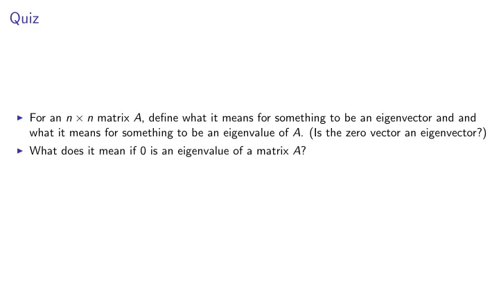
Quiz I For an n × n matrix A , define what it means for something to be an eigenvector and and what it means for something to be an eigenvalue of A . (Is the zero vector an eigenvector?) I What does it mean if 0 is an eigenvalue of a matrix A ?

Not for credit Suppose A is an n × n matrix, and suppose v 1 , . . . , v n are eigenvectors that form a basis for R n . Let v be a vector in R n . Suppose that the coordinate representation of v in terms of v 1 , . . . , v n is [ ↵ 1 , . . . , ↵ n ]. What is the coordinate representation of A v ?

Interpretation using change of basis, revisited A diagonalizable ⇒ A = S Λ S � 1 for a diag. Λ and invertible S . Suppose x (0) is a vector. The equation x ( t +1) = A x ( t ) then defines x (1) , x (2) , x (3) , . . . . Then x ( t ) x (0) = A A · · · A | {z } t times ( S Λ S � 1 )( S Λ S � 1 ) · · · ( S Λ S � 1 ) x (0) = S Λ t S � 1 x (0) = Interpretation: Let u ( t ) = coordinate representation of x ( t ) in terms of the columns of S . Then we have the equation u ( t +1) = Λ u ( t ) . Therefore 2 3 � 1 ... 5 then If Λ = 4 u ( t ) u (0) � n = Λ Λ · · · Λ | {z } 2 3 � t 1 ... t times Λ t = Λ t u (0) 4 5 = � t n

Interpretation using change of basis, re-revisited Suppose n × n matrix A is diagonalizable, so it has linearly independent e-vectors v 1 , v 2 , . . . , v n with e-values are � 1 ≥ � 2 ≥ . . . ≥ � n . Any vector x can be written as a linear combination: x = ↵ 1 v 1 + · · · + ↵ n v n Left-multiply by A on both sides of the equation: A x = A ( ↵ 1 v 1 ) + A ( ↵ 2 v 2 ) + · · · + A ( ↵ n v n ) ↵ 1 A v 1 + ↵ 2 A v 2 + · · · + ↵ n A v n = = ↵ 1 � 1 v 1 + ↵ 2 � 2 v 2 + · · · + ↵ n � n v n Applying the same reasoning to A ( A x ), we get A 2 x = ↵ 1 � 2 1 v 1 + ↵ 2 � 2 2 v 2 + · · · + ↵ n � 2 n v n More generally, for any nonnegative integer t , A t x = ↵ 1 � t 1 v 1 + ↵ 2 � t 2 v 2 + · · · + ↵ n � t n v n If | � 1 | > | � 2 | then eventually � t 1 will be much bigger than � t 2 , . . . , � t n , so first term will dominate. For a large enough value of t , A t x will be approximately ↵ 1 � t 1 v 1 .

Rabbit reproduction and death A disease enters the rabbit population. In each month, I A � fraction of the adult population catches it, I an ✏ fraction of the juvenile population catches it, and I an ⌘ fraction of the sick population die, and the rest recover. Sick rabbits don’t produce babies. Equations well adults 0 = (1 − � ) well adults + (1 − ✏ )juveniles + (1 − ⌘ ) sick juveniles 0 = well adults sick 0 = � well adults + ✏ juveniles + 0 Represent change in populations by matrix-vector equation 2 3 2 3 2 3 well adults at time t + 1 1 − � 1 − ✏ (1 − ⌘ ) well adults at time t 5 = juveniles at time t + 1 1 0 0 juveniles at time t 4 4 5 4 5 sick at time t + 1 0 sick at time t � ✏ (You might question fractional rabbits, deterministic infection.) Question: Does the rabbit population still grow?

Analyzing the rabbit population in the presence of disease 2 3 2 3 2 3 well adults at time t + 1 1 − � 1 − ✏ (1 − ⌘ ) well adults at time t 5 = juveniles at time t + 1 1 0 0 juveniles at time t 4 4 5 4 5 sick at time t + 1 � ✏ 0 sick at time t Question: Does the rabbit population still grow? Depends on the values of the parameters ( � = infection rate among adults, ✏ = infection rate among juveniles, ⌘ = death rate among sick). Plug in di ff erent values for parameters and then compute eigenvalues I � = 0 . 5 , ✏ = 0 . 5 , ⌘ = 0 . 8. The largest eigenvalue is 1.1172 (with eigenvector [0 . 6299 , 0 . 5638 , 0 . 5342]). This means that the population grows exponentially in time (roughly proportional to 1 . 117 t ). I � = 0 . 7 , ✏ = 0 . 7 , ⌘ = 0 . 8. The largest eigenvalue is 0.9327. This means the population shrinks exponentially. I � = 0 . 6 , ✏ = 0 . 6 , ⌘ = 0 . 8. The largest eigenvalue is 1.02. Population grows exponentially.

Expected number of rabbits There’s these issues of fractional rabbits and deterministic disease. The matrix-vector equation really describes the expected values of the various populations.

Modeling population movement Dance-club dynamics: At the beginning of each song, I 56% of the people standing on the side go onto the dance floor, and I 12% of the people on the dance floor leave it. Suppose that there are a hundred people in the club. Assume nobody enters the club and nobody leaves. What happens to the number of people in each of the two locations? Represent state of system by  number of people standing on side after t songs " # � x ( t ) x ( t ) = 1 = x ( t ) number of people on dance floor after t songs 2  . 44 " # � " # x ( t +1) x ( t ) . 12 1 1 = x ( t +1) x ( t ) . 56 . 88 2 2 Diagonalize: S � 1 AS = Λ where  . 44  0 . 209529  1 � � � . 12 − 1 0 A = , S = , Λ = . 56 . 88 0 . 977802 1 0 0 . 32

Analyzing dance-floor dynamics " # " # x ( t ) x (0) � S Λ S � 1 � t 1 1 = x ( t ) x (0) 2 2 " # x (0) S Λ t S � 1 1 = x (0) 2  . 21 �  1 � " # � t  x (0) − 1 0 . 84 . 84 1 = x (0) . 98 1 0 . 32 − . 82 . 18 2  . 21 �  1 t � " # �  x (0) − 1 0 . 84 . 84 1 = x (0) . 98 1 0 . 32 t − . 82 . 18 2  . 21  − 1 � � 1 t ( . 84 x (0) + . 84 x (0) + (0 . 32) t ( − . 82 x (0) + . 18 x (0) = 2 ) 2 ) 1 1 . 98 1  . 18 ⌘  − 1 � � 1 t ⇣ ⌘ + (0 . 32) t ⇣ x (0) + x (0) − . 82 x (0) + . 18 x (0) = 1 2 1 2 . 82 1 | {z } total population

Analyzing dance-floor dynamics, continued  . 18 " # ⌘  − 1 x ( t ) � � ⇣ ⌘ + (0 . 32) t ⇣ x (0) + x (0) − . 82 x (0) + . 18 x (0) 1 = x ( t ) 1 2 1 2 . 82 1 2 | {z } total population The numbers of people in the two locations after t songs depend on the initial numbers of people in the two locations. However, the dependency grows weaker as the number of songs increases: (0 . 32) t gets smaller and smaller, so the second term in the sum matters less and less. After ten songs, (0 . 32) t is about 0.00001.  . 18 � The first term in the sum is times the total number of people. This shows that, as the . 82 number of songs increases, the proportion of people on the dance floor gets closer and closer to 82%.

Modeling Randy Without changing math, we switch interpretations. Instead of modeling whole dance-club population, we model one person, Randy. Randy’s behavior captured in transition diagram: 0.56 0.44 S1 S2 0.88 0.12 State S1 represents Randy being on the side. State S2 represents Randy being on the dance floor. After each song, Randy follows one of the arrows from current state. Which arrow? Chosen randomly according to probabilities on the arrows ( transition probabilities ). For each state, labels on arrows from that state must sum to 1.

Where is Randy? Knowing where Randy starts at time 0 doesn’t let us predict with certainty where he will be at time t . However, for each time t , we can calculate the probability distribution for his location. Since there are two possible locations (o ff floor, on floor), the probability distribution is given by " # x ( t ) a 2-vector x ( t ) = where x ( t ) + x ( t ) 1 = 1. x ( t ) 1 2 2 Probability distribution for Randy’s location at time t + 1 is related to probability distribution for Randy’s location at time t :  . 44 " # � " # x ( t +1) x ( t ) . 12 1 1 = x ( t +1) x ( t ) . 56 . 88 2 2 Using earlier analysis, ⌘  . 18 " # ⌘  − 1 � � x ( t ) ⇣ + (0 . 32) t ⇣ x (0) + x (0) − . 82 x (0) + . 18 x (0) 1 = x ( t ) 1 2 1 2 . 82 1 2  . 18 ⌘  − 1 � � + (0 . 32) t ⇣ − . 82 x (0) + . 18 x (0) = 1 2 . 82 1

Where is Randy?  . 18 " # ⌘  − 1 � � x ( t ) + (0 . 32) t ⇣ − . 82 x (0) + . 18 x (0) 1 = x ( t ) 1 2 . 82 1 2 If we know Randy starts o ff the dance floor at time 0 then x (0) = 1 and x (0) = 0. 1 2 If we know Randy starts on the dance floor at time 0 then x (0) = 0 and x (0) = 1. 1 2 In either case, we can plug in to equation to get exact probability distribution for time t . But after a few songs, the starting location doesn’t matter much—the probability distribution  . 18 � gets very close to in either case. . 82 This is called Randy’s stationary distribution . It doesn’t mean Randy stays in one place—we expect him to move back and forth all the time. It means that the probability distribution for his location after t steps depends less and less on t .

From Randy to spatial locality in CPU memory fetches We again switch interpretations without changing the math. CPU uses caches and prefetching to improve performance. To help computer architects, it is useful to model CPU access patterns. After accessing location x , CPU usually accesses location x + 1. Therefore simple model is: Probability[address requested at time t + 1 is 1 + address requested at time t ] = . 6 However, a slightly more sophisticated model predicts much more accurately. Observation: Once consecutive addresses have been requested in timesteps t and t + 1, it is very likely that the address requested in timestep t + 2 is also consecutive. Use same model as used for Randy. 0.56 State S1 = CPU is requesting nonconsecutive addresses. 0.44 S1 S2 0.88 State S2 = CPU is requesting consecutive addresses. 0.12