Efficient Parameter-Estimating Often, the Empirical . . . - PowerPoint PPT Presentation
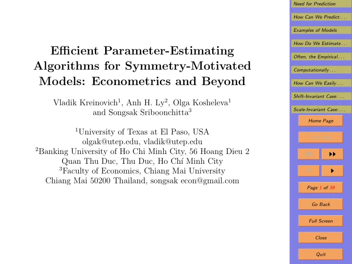
Need for Prediction How Can We Predict: . . . Examples of Models How Do We Estimate . . . Efficient Parameter-Estimating Often, the Empirical . . . Algorithms for Symmetry-Motivated Computationally . . . Models: Econometrics and Beyond How
Need for Prediction How Can We Predict: . . . Examples of Models How Do We Estimate . . . Efficient Parameter-Estimating Often, the Empirical . . . Algorithms for Symmetry-Motivated Computationally . . . Models: Econometrics and Beyond How Can We Easily . . . Shift-Invariant Case: . . . Vladik Kreinovich 1 , Anh H. Ly 2 , Olga Kosheleva 1 Scale-Invariant Case: . . . and Songsak Sriboonchitta 3 Home Page 1 University of Texas at El Paso, USA Title Page olgak@utep.edu, vladik@utep.edu 2 Banking University of Ho Chi Minh City, 56 Hoang Dieu 2 ◭◭ ◮◮ Quan Thu Duc, Thu Duc, Ho Ch´ ı Minh City 3 Faculty of Economics, Chiang Mai University ◭ ◮ Chiang Mai 50200 Thailand, songsak econ@gmail.com Page 1 of 39 Go Back Full Screen Close Quit
Need for Prediction How Can We Predict: . . . 1. Need for Prediction Examples of Models • In many real-life situations, we have a quantity x that How Do We Estimate . . . changes with time t . Often, the Empirical . . . Computationally . . . • We want to use the previous values of this quantity to How Can We Easily . . . predict its future values. Shift-Invariant Case: . . . • For example: Scale-Invariant Case: . . . – we know how the stock price has changed with time, Home Page and Title Page – we want to use this information to predict future ◭◭ ◮◮ stock prices. ◭ ◮ • In many cases, such a prediction is possible; for exam- Page 2 of 39 ple: Go Back – when weather records show clear yearly cycles, Full Screen – it is reasonable to predict that a similar yearly cycle will be observed in the future as well. Close Quit
Need for Prediction How Can We Predict: . . . 2. How Can We Predict: Main Idea Examples of Models • A usual approach to prediction is that we select some How Do We Estimate . . . model , i.e., some parametric family of functions Often, the Empirical . . . Computationally . . . f ( t, c 1 , . . . , c ℓ ) . How Can We Easily . . . • Based on the available observations, we find the pa- Shift-Invariant Case: . . . rameters � c i which provide the best fit. Scale-Invariant Case: . . . Home Page • hen we use these values � c j to predict the future values Title Page of the quantity x as x ( t ) ≈ f ( t, � c 1 , . . . , � c ℓ ) . ◭◭ ◮◮ ◭ ◮ Page 3 of 39 Go Back Full Screen Close Quit
Need for Prediction How Can We Predict: . . . 3. Examples of Models Examples of Models • In some cases, the dependence of the quantity x on How Do We Estimate . . . time t is polynomial, in which case Often, the Empirical . . . f ( t, c 1 , . . . , c ℓ ) = c 1 + c 2 · t + c 3 · t 2 + . . . + c ℓ · t ℓ − 1 . Computationally . . . How Can We Easily . . . • For a simple periodic process, the dependence of the Shift-Invariant Case: . . . quantity x on time is described by a sinusoid: Scale-Invariant Case: . . . Home Page f ( t, c 1 , c 2 , c 3 ) = c 1 · sin( c 2 · t + c 3 ) . Title Page • To get a more realistic description of a periodic process, ◭◭ ◮◮ we need to take into account higher harmonics: ◭ ◮ f ( t, c 1 , c 2 , . . . ) = c 1 · sin( c 2 · t + c 3 )+ c 4 · sin(2 c 2 · t + c 5 )+ . . . Page 4 of 39 • For a simple radioactive decay, the amount of radioac- Go Back tive material decreases exponentially: Full Screen f ( t, c 1 , c 2 ) = c 1 · exp( − c 2 · t ) . Close Quit
Need for Prediction How Can We Predict: . . . 4. Examples of Models (cont-d) Examples of Models • A more realistic model is a mixture of several different How Do We Estimate . . . isotopes, with different half-lives: Often, the Empirical . . . Computationally . . . f ( t, c 1 , c 2 , . . . ) = c 1 · exp( − c 2 · t ) + c 3 · exp( − c 4 · t ) + . . . How Can We Easily . . . Shift-Invariant Case: . . . • Other models include log-periodic model which is used to predict economic crashes: Scale-Invariant Case: . . . Home Page c 1 + c 2 · ( c 3 − t ) c 4 + c 5 · ( c 3 − t ) c 4 · cos( c 6 · ln( c 3 − t ) + c 7 ) . Title Page • The following software model describes the number of ◭◭ ◮◮ bugs discovered by time t : ◭ ◮ f ( t, c 1 , c 2 , c 3 ) = c 1 · ln( t − c 2 ) + c 3 . Page 5 of 39 Go Back • A more complex example is a neural network, when c j are the corresponding weights. Full Screen Close Quit
Need for Prediction How Can We Predict: . . . 5. How Do We Estimate the Parameters? Examples of Models • Usually, the Least Squares method is used to estimate How Do We Estimate . . . the values of the parameters c 1 , . . . , c ℓ . Often, the Empirical . . . Computationally . . . • So, based on the observed values x ( t i ), we find c j that � n How Can We Easily . . . ( x i − f ( t i , c 1 , . . . , c ℓ )) 2 . minimize Shift-Invariant Case: . . . i =1 Scale-Invariant Case: . . . • In some cases – e.g., for the polynomial dependence – Home Page the model f ( x, c 1 , . . . , c ℓ ) linearly depends on c j . Title Page • Then, the minimized expression is quadratic in c j . ◭◭ ◮◮ • We can find the minimum of a function of several vari- ◭ ◮ ables by equating all its partial derivatives to 0. Page 6 of 39 • For a quadratic objective function, all the partial Go Back derivatives are linear functions of c j . Full Screen Close Quit
Need for Prediction How Can We Predict: . . . 6. How Do We Estimate the Parameters (cont-d) Examples of Models • Thus, by equating them all to 0, we get a system of How Do We Estimate . . . linear equations for the unknowns c j . Often, the Empirical . . . Computationally . . . • For solving systems of linear equations, there are many How Can We Easily . . . efficient algorithms. Shift-Invariant Case: . . . • So in this case, the problem of identifying the model’s Scale-Invariant Case: . . . parameters is computationally easy. Home Page • On the other hand, in general, the dependence of the Title Page model on the parameters c j is non-linear. ◭◭ ◮◮ • Thus, the objective function is more complex than ◭ ◮ quadratic. Page 7 of 39 • It is known that, in general, optimization is computa- Go Back tionally intensive – NP-hard. Full Screen • It is therefore desirable to select models for which iden- tification is easier. But how do we select modles? Close Quit
Need for Prediction How Can We Predict: . . . 7. How Are Models Selected in the First Place? Examples of Models • Sometimes, we have an good understanding of the pro- How Do We Estimate . . . cesses that cause the quantity x to change. Often, the Empirical . . . Computationally . . . • In such situations, we have a theoretically justified How Can We Easily . . . model. Shift-Invariant Case: . . . • In most cases, however, the model is selected empiri- Scale-Invariant Case: . . . cally: Home Page – we try different models, and Title Page – we select the one for which, for the same number ◭◭ ◮◮ of parameters, the approximation error is min. ◭ ◮ Page 8 of 39 Go Back Full Screen Close Quit
Need for Prediction How Can We Predict: . . . 8. Often, the Empirical Efficiency of Selected Examples of Models Models Can Be Explained by Symmetry How Do We Estimate . . . • In an empirical choice, we only compare a few possible Often, the Empirical . . . models. Computationally . . . How Can We Easily . . . • As a result Shift-Invariant Case: . . . – the fact that the selected model turned out to be Scale-Invariant Case: . . . better than others Home Page – does not necessarily mean that this model is indeed Title Page the best for a given phenomenon: ◭◭ ◮◮ – there are, in principle, many other models that we ◭ ◮ did not consider in our empirical comparison. Page 9 of 39 • Good news is that in many cases, the empirical selec- tion can be confirmed by a theoretical analysis. Go Back • Often, the empirically successful model can be derived Full Screen from the natural symmetry requirements. Close Quit
Need for Prediction How Can We Predict: . . . 9. But the Model Remains Computationally In- Examples of Models tensive How Do We Estimate . . . • The fact that the empirically selected model is theo- Often, the Empirical . . . retically justified does not change its formulas; so: Computationally . . . How Can We Easily . . . – if the dependence of this model on the correspond- Shift-Invariant Case: . . . ing parameters c j is non-linear, Scale-Invariant Case: . . . – the problem of identifying parameters of this model Home Page remains computationally intensive. Title Page • In this talk, we show that symmetries: ◭◭ ◮◮ – are not only helpful in selecting a model, ◭ ◮ – they can also help design computationally efficient Page 10 of 39 algorithms for identifying model’s parameters. Go Back Full Screen Close Quit
Recommend
More recommend
Explore More Topics
Stay informed with curated content and fresh updates.
