Econometrics 2 Combine cross sections obtained at different points - PowerPoint PPT Presentation
Pooled Cross Sections and Panel Data Last time: Pooling independent cross sections across time (13.1-2). Econometrics 2 Combine cross sections obtained at different points in time. Partial pooling: Allow the coefficients of some
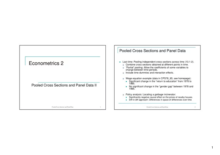
Pooled Cross Sections and Panel Data Last time: Pooling independent cross sections across time (13.1-2). � Econometrics 2 � Combine cross sections obtained at different points in time. � ”Partial” pooling: Allow the coefficients of some variables to change between time periods. � Include time dummies and interaction effects. � Wage equation example (data in CPS78_85, see homepage): Significant change in the ”return to education” from 1978 to � 1985. Pooled Cross Sections and Panel Data II No significant change in the ”gender gap” between 1978 and � 1985. � Policy analysis: Locating a garbage incinerator: Significantly negative causal effect on the prices of nearby houses. � Diff-in-diff approach: Differences in space of differences over time � Pooled Cross Sections and Panel Data 1 Pooled Cross Sections and Panel Data 2 1
Pooled Cross Sections and Panel Data Data structure � Panel data : Same n individuals in period 1 and period 2. = ( y , x , x ,..., x ), i 1,2,..., n � Period 1: Today: Two-period panel data: Follow the same individuals i 1 i 11 i 12 i k 1 = � Period 2: ( y , x , x ,..., x ), i 1,2,..., n over two periods (13.3-4) 2 21 22 2 i i i i k � Total of 2n observations on n individuals � Period 2 could be some years (months, weeks, …) after period 1 � Unobserved effects model: Time-invariant and idiosyncratic effects � Omitted variables bias (heterogeneity bias) � Also called longitudinal data. � First-difference estimation � Policy analysis with two-period panel data � Simple case: One regressor. Simply want to estimate the effect of x on y. Pooled Cross Sections and Panel Data 3 Pooled Cross Sections and Panel Data 4 2
Unobserved effects model Assumptions on the composite error term = + = β + δ + β + + v a u y d 2 x a u � Model: � Composite error term: i 0 0 t 1 it i it it i it d � Time dummy: Same values for all individuals � Assume that (conditional on the regressors): 2 t = = = � Composite error term: E u ( ) 0, i 1,2,..., , n t 1,2 = + v a u it it i it = ≠ = E u u ( ) 0, for all i j , t 1,2 it jt a � Unobserved fixed effect (unobserved heterogeneity): = = = i E u a ( ) 0, i 1,2,..., , n t 1,2 it i � Time-invariant = = E u x ( ) 0, for all , and s, i j t 1,2 � Specific to each individual it jt u � Idiosyncratic error: � Note: We will make no assumption on (for now). it E a x ( ) i it � Varies over individuals and time: ”Regular” error term Pooled Cross Sections and Panel Data 5 Pooled Cross Sections and Panel Data 6 3
Correlated unobserved heterogeneity First-difference estimation = β + δ + β + + a y d 2 x a u � Unobserved time-invariant effect could well be Model: � i 0 0 t 1 it i it i ≠ correlated with the observed variable: E a x ( ) 0 i it = β + δ + β + + Period 2: y ( ) x a u � Pooling the observations and estimating the model by OLS: i 2 0 0 1 i 2 i i 2 = β + β + + Period 1: y x a u Will result in inconsistent estimates. i 1 0 1 i 1 i i 1 � Problem cannot be solved if the available data is just a single − = δ + β − + − x y cross section of information on and First-differencing: ( ) y y x x u u it it i 2 i 1 0 1 i 2 i 1 i 2 i 1 ⇔ ∆ = δ + β ∆ + ∆ � Fixed effect panel data solution: Estimate a model in which: y x u i 2 0 1 i 2 i 2 β � The parameter of interest, , is identified 1 a � The fixed effects, , does not appear. a The unobserved fixed effect is ”differenced” away. � i i We have a cross section of first differences that allows us to � One such method is first-differencing . � β u estimate consistently (given the assumptions on ). it 1 Pooled Cross Sections and Panel Data 7 Pooled Cross Sections and Panel Data 8 4
First-difference estimation First-difference estimation � More general case: Several observed regressors, some Example: Wage equation for prime-age male workers may be time-invariant ∆ = δ + β ∆ + β ∆ + ∆ First-differenced model: y x x u i 2 0 1 i 12 2 i 22 i 2 Example: Wage equation for prime-age male workers Note: * The time-invariant variable, years of education, has been differenced out y the log of wage for worker in period i t it β along with the fixed effect. Cannot estimate . x local unemployment rate for worker in period i t 3 it 1 ∆ * The variable x will be equal to 12 for most workers, less than 12 if x experience (months working) for worker in peri i od t i 22 it 2 β individual has been unemployed. If little variation over workers then x number of years of education for worker (time-invariant) i 2 i 3 will be imprecisely estimated (large standard errors). a "ability" for worker (time-invariant) i i * First-differenced estimates could be very different from pooled cross-sectional estimates: Indicates important heterogeneity bias. ∆ = δ + β ∆ + β ∆ + ∆ First-differenced model: y x x u i 2 0 1 i 12 2 i 22 i 2 Pooled Cross Sections and Panel Data 9 Pooled Cross Sections and Panel Data 10 5
Policy analysis with panel data (treatment effects) Policy analysis with panel data � Panel data even more useful for policy analysis than a time series of cross sections. = β + δ + β + � Model: y d 2 prog v i 0 0 t 1 it it � Program evaluation: � Note: � Want to measure the causal effect of an individual participating in � Similar to model used for independent cross sections some programme ”Active labour market policy” programme � � Panel data allows error component structure: Subsidies to firms to make them innovate, become more productive, � = + v a u export, …. it i it � Potential problem: � Control for time-invariant characteristics of Individuals select into the program prog = � participants ( ) and 1 � it Or they are assigned to the program � prog = non-participants ( ) 0 � it based on individual characteristics that are related to the outcome including variables that are likely to affect the participation variable. decision. � Outcome measures: Post-programme wage, R&D expenses, productivity, export intensity, … Pooled Cross Sections and Panel Data 11 Pooled Cross Sections and Panel Data 12 6
Policy analysis with panel data Policy analysis with panel data: Example First-differenced model: � Example: The effect of a grant to firms for job training. � ∆ = δ + β + ∆ � Aim of program: Enhance the productivity of workers in i y prog u 2 0 1 i 2 i 2 the firm. If participation only in period 2 (”before-after”) the OLS estimate � � Effect measure: ”Scrap rate” (proportion of produced becomes simply items that have defects): β = ∆ − ∆ ˆ y y � Many defects = low average level of productivity in the firm − 1 part non part � Few defects = high productivity. Diff-in-diff estimate. � � Model: a Panel structure: No assumption needed on � i = β + δ + β + + ∆ scrap d 88 grant a u prog Still need to assume that u and are uncorrelated for � it 0 0 t 1 it i it it it consistency. � How can we obtain a consistent estimate of any causal Review the incinerator example. β � effect, ? 1 Pooled Cross Sections and Panel Data 13 Pooled Cross Sections and Panel Data 14 7
Policy analysis with panel data: Example Policy analysis with panel data: Example � Problem: � Questions: � Participation may be related to unobserved firm effects (worker � Are there indications of heterogeneity bias and manager ability, the amount of capital available,…). here? � Unobserved effects likely to be directly related to productivity. � OLS on pooled set of observations: � What is the likely direction of any bias? � = − + = = � How do firms select into the job training 2 log( ) 0.597 0.189 88 0.057 108, 0.0034 scrap d grant n R it t it program? (0.205) (0.328) (0.431) � Diff-in-diff approach: � ∆ = − − ∆ = = 2 log( scrap ) 0.057 0.317 grant n 54, R 0.067 it it (0.097) (0.164) Pooled Cross Sections and Panel Data 15 Pooled Cross Sections and Panel Data 16 8
Next time � Thursday this week! � Panel data with several observations over time for the same individual units. � W sec. 13.5, 14.1. � Exercises start this week! Pooled Cross Sections and Panel Data 17 9
Recommend
More recommend
Explore More Topics
Stay informed with curated content and fresh updates.
