Dynamic Programming Lecturer: Shi Li Department of Computer Science - PowerPoint PPT Presentation
CSE 431/531: Analysis of Algorithms Dynamic Programming Lecturer: Shi Li Department of Computer Science and Engineering University at Buffalo Paradigms for Designing Algorithms Greedy algorithm Make a greedy choice Prove that the greedy
CSE 431/531: Analysis of Algorithms Dynamic Programming Lecturer: Shi Li Department of Computer Science and Engineering University at Buffalo
Paradigms for Designing Algorithms Greedy algorithm Make a greedy choice Prove that the greedy choice is safe Reduce the problem to a sub-problem and solve it iteratively Divide-and-conquer Break a problem into many independent sub-problems Solve each sub-problem separately Combine solutions for sub-problems to form a solution for the original one Usually used to design more efficient algorithms 2/99
Paradigms for Designing Algorithms Dynamic Programming Break up a problem into many overlapping sub-problems Build solutions for larger and larger sub-problems Use a table to store solutions for sub-problems for reuse 3/99
Recall: Computing the n -th Fibonacci Number F 0 = 0 , F 1 = 1 F n = F n − 1 + F n − 2 , ∀ n ≥ 2 Fibonacci sequence: 0 , 1 , 1 , 2 , 3 , 5 , 8 , 13 , 21 , 34 , 55 , 89 , · · · Fib( n ) F [0] ← 0 1 F [1] ← 1 2 for i ← 2 to n do 3 F [ i ] ← F [ i − 1] + F [ i − 2] 4 return F [ n ] 5 Store each F [ i ] for future use. 4/99
Outline Weighted Interval Scheduling 1 Subset Sum Problem 2 Knapsack Problem 3 Longest Common Subsequence 4 Longest Common Subsequence in Linear Space Shortest Paths in Graphs with Negative Weights 5 Shortest Paths in Directed Acyclic Graphs Bellman-Ford Algorithm All-Pair Shortest Paths and Floyd-Warshall 6 Matrix Chain Multiplication 7 Summary 8 5/99
Recall: Interval Schduling Input: n jobs, job i with start time s i and finish time f i each job has a weight (or value) v i > 0 i and j are compatible if [ s i , f i ) and [ s j , f j ) are disjoint Output: a maximum-size subset of mutually compatible jobs 0 1 2 3 4 5 6 7 8 9 100 50 30 25 50 90 80 80 70 Optimum value = 220 6/99
Hard to Design a Greedy Algorithm Q: Which job is safe to schedule? Job with the earliest finish time? No, we are ignoring weights Job with the largest weight? No, we are ignoring times Job with the largest weight length ? No, when weights are equal, this is the shortest job 0 1 2 3 4 5 6 7 8 9 7/99
Designing a Dynamic Programming Algorithm i opt [ i ] 0 1 2 3 4 5 6 7 8 9 0 0 5 2 100 50 9 30 1 80 4 25 8 50 2 100 3 90 7 80 3 100 1 80 6 70 4 105 5 150 6 170 Sort jobs according to non-decreasing 7 185 order of finish times 8 220 opt [ i ] : optimal value for instance only 9 220 containing jobs { 1 , 2 , · · · , i } 8/99
Designing a Dynamic Programming Algorithm Focus on instance 0 1 2 3 4 5 6 7 8 9 { 1 , 2 , 3 , · · · , i } , 2 100 5 50 9 30 opt [ i ] : optimal value for the 25 50 4 8 instance 3 90 7 80 assume we have computed 1 80 6 70 opt [0] , opt [1] , · · · , opt [ i − 1] Q: The value of optimal solution that does not contain i ? A: opt [ i − 1] Q: The value of optimal solution that contains job i ? A: v i + opt [ p i ] , p i = the largest j such that f j ≤ s i 9/99
Designing a Dynamic Programming Algorithm Q: The value of optimal solution that does not contain i ? A: opt [ i − 1] Q: The value of optimal solution that contains job i ? A: v i + opt [ p i ] , p i = the largest j such that f j ≤ s i Recursion for opt [ i ] : opt [ i ] = max { opt [ i − 1] , v i + opt [ p i ] } 10/99
Designing a Dynamic Programming Algorithm Recursion for opt [ i ] : opt [ i ] = max { opt [ i − 1] , v i + opt [ p i ] } 0 1 2 3 4 5 6 7 8 9 2 100 5 50 9 30 4 25 8 50 3 90 7 80 1 80 6 70 opt [0] = 0 opt [1] = max { opt [0] , 80 + opt [0] } = 80 opt [2] = max { opt [1] , 100 + opt [0] } = 100 opt [3] = max { opt [2] , 90 + opt [0] } = 100 opt [4] = max { opt [3] , 25 + opt [1] } = 105 opt [5] = max { opt [4] , 50 + opt [3] } = 150 11/99
Designing a Dynamic Programming Algorithm Recursion for opt [ i ] : opt [ i ] = max { opt [ i − 1] , v i + opt [ p i ] } 0 1 2 3 4 5 6 7 8 9 2 100 5 50 9 30 4 25 8 50 3 90 7 80 1 80 6 70 opt [0] = 0 , opt [1] = 80 , opt [2] = 100 opt [3] = 100 , opt [4] = 105 , opt [5] = 150 opt [6] = max { opt [5] , 70 + opt [3] } = 170 opt [7] = max { opt [6] , 80 + opt [4] } = 185 opt [8] = max { opt [7] , 50 + opt [6] } = 220 opt [9] = max { opt [8] , 30 + opt [7] } = 220 12/99
Recursive Algorithm to Compute opt [ n ] sort jobs by non-decreasing order of finishing times 1 compute p 1 , p 2 , · · · , p n 2 return compute-opt ( n ) 3 compute-opt ( i ) if i = 0 then 1 return 0 2 else 3 return max { compute-opt ( i − 1) , v i + compute-opt ( p i ) } 4 Running time can be exponential in n Reason: we are computed each opt [ i ] many times Solution: store the value of opt [ i ] , so it’s computed only once 13/99
Memoized Recursive Algorithm sort jobs by non-decreasing order of finishing times 1 compute p 1 , p 2 , · · · , p n 2 opt [0] ← 0 and opt [ i ] ← ⊥ for every i = 1 , 2 , 3 , · · · , n 3 return compute-opt ( n ) 4 compute-opt ( i ) if opt [ i ] = ⊥ then 1 opt [ i ] ← max { compute-opt ( i − 1) , v i + compute-opt ( p i ) } 2 return opt [ i ] 3 Running time sorting: O ( n lg n ) Running time for computing p : O ( n lg n ) via binary search Running time for computing opt [ n ] : O ( n ) 14/99
Dynamic Programming sort jobs by non-decreasing order of finishing times 1 compute p 1 , p 2 , · · · , p n 2 opt [0] ← 0 3 for i ← 1 to n 4 opt [ i ] ← max { opt [ i − 1] , v i + opt [ p i ] } 5 Running time sorting: O ( n lg n ) Running time for computing p : O ( n lg n ) via binary search Running time for computing opt [ n ] : O ( n ) 15/99
How Can We Recover the Optimum Schedule? sort jobs by non-decreasing order 1 of finishing times i ← n, S ← ∅ 1 compute p 1 , p 2 , · · · , p n 2 while i � = 0 2 opt [0] ← 0 3 if b [ i ] = N 3 for i ← 1 to n 4 i ← i − 1 4 if opt [ i − 1] ≥ v i + opt [ p i ] 5 else 5 opt [ i ] ← opt [ i − 1] 6 S ← S ∪ { i } 6 b [ i ] ← N 7 i ← p i 7 else 8 return S 8 opt [ i ] ← v i + opt [ p i ] 9 b [ i ] ← Y 10 16/99
Recovering Optimum Schedule: Example i opt [ i ] b [ i ] 0 0 ⊥ 1 80 Y 0 1 2 3 4 5 6 7 8 9 2 100 Y 3 100 N 2 100 5 50 9 30 4 105 Y 4 25 8 50 5 150 Y 3 90 7 80 i 6 170 Y 80 70 1 6 7 185 Y 8 220 Y 9 220 N 17/99
Dynamic Programming Break up a problem into many overlapping sub-problems Build solutions for larger and larger sub-problems Use a table to store solutions for sub-problems for reuse 18/99
Outline Weighted Interval Scheduling 1 Subset Sum Problem 2 Knapsack Problem 3 Longest Common Subsequence 4 Longest Common Subsequence in Linear Space Shortest Paths in Graphs with Negative Weights 5 Shortest Paths in Directed Acyclic Graphs Bellman-Ford Algorithm All-Pair Shortest Paths and Floyd-Warshall 6 Matrix Chain Multiplication 7 Summary 8 19/99
Subset Sum Problem Input: an integer bound W > 0 a set of n items, each with an integer weight w i > 0 Output: a subset S of items that � � maximizes w i s.t. w i ≤ W. i ∈ S i ∈ S Motivation: you have budget W , and want to buy a subset of items, so as to spend as much money as possible. Example: W = 35 , n = 5 , w = (14 , 9 , 17 , 10 , 13) Optimum: S = { 1 , 2 , 4 } and 14 + 9 + 10 = 33 20/99
Greedy Algorithms for Subset Sum Candidate Algorithm: Sort according to non-increasing order of weights Select items in the order as long as the total weight remains below W Q: Does candidate algorithm always produce optimal solutions? A: No. W = 100 , n = 3 , w = (51 , 50 , 50) . Q: What if we change “non-increasing” to “non-decreasing”? A: No. W = 100 , n = 3 , w = (1 , 50 , 50) 21/99
Design a Dynamic Programming Algorithm Consider the instance: i, W ′ , ( w 1 , w 2 , · · · , w i ) ; opt [ i, W ′ ] : the optimum value of the instance Q: The value of the optimum solution that does not contain i ? A: opt [ i − 1 , W ′ ] Q: The value of the optimum solution that contains i ? A: opt [ i − 1 , W ′ − w i ] + w i 22/99
Dynamic Programming Consider the instance: i, W ′ , ( w 1 , w 2 , · · · , w i ) ; opt [ i, W ′ ] : the optimum value of the instance 0 i = 0 opt [ i − 1 , W ′ ] i > 0 , w i > W ′ opt [ i, W ′ ] = � � opt [ i − 1 , W ′ ] i > 0 , w i ≤ W ′ max opt [ i − 1 , W ′ − w i ] + w i 23/99
Dynamic Programming for W ′ ← 0 to W 1 opt [0 , W ′ ] ← 0 2 for i ← 1 to n 3 for W ′ ← 0 to W 4 opt [ i, W ′ ] ← opt [ i − 1 , W ′ ] 5 if w i ≥ W ′ and opt [ i − 1 , W ′ − w i ] + w i ≥ opt [ i, W ′ ] 6 then opt [ i, W ′ ] ← opt [ i − 1 , W ′ − w i ] + w i 7 return opt [ n, W ] 8 24/99
Recover the Optimum Set for W ′ ← 0 to W 1 opt [0 , W ′ ] ← 0 2 for i ← 1 to n 3 for W ′ ← 0 to W 4 opt [ i, W ′ ] ← opt [ i − 1 , W ′ ] 5 b [ i, W ′ ] ← N 6 if w i ≤ W ′ and opt [ i − 1 , W ′ − w i ] + w i ≥ opt [ i, W ′ ] 7 then opt [ i, W ′ ] ← opt [ i − 1 , W ′ − w i ] + w i 8 b [ i, W ′ ] ← Y 9 10 return opt [ n, W ] 25/99
Recover the Optimum Set i ← n, W ′ ← W, S ← ∅ 1 while i > 0 2 if b [ i, W ′ ] = Y then 3 W ′ ← W ′ − w i 4 S ← S ∪ { i } 5 i ← i − 1 6 return S 7 26/99
Recommend
More recommend
Explore More Topics
Stay informed with curated content and fresh updates.

![COMMUNICATING [with empathy] @ DY DYNAMIC JILL JILL @ DY DYNAMIC JILL TENSION IS INEVITABLE @](https://c.sambuz.com/548934/communicating-s.webp)

