Acknowledgement The set of slides have use materials from the - PowerPoint PPT Presentation

Acknowledgement • The set of slides have use materials from the Graph: representation and traversal 
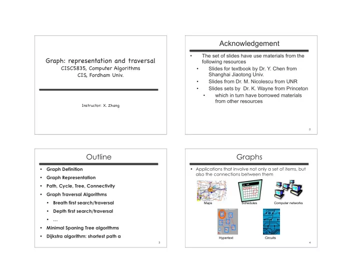
 following resources CISC5835, Computer Algorithms • Slides for textbook by Dr. Y. Chen from CIS, Fordham Univ. Shanghai Jiaotong Univ. • Slides from Dr. M. Nicolescu from UNR • Slides sets by Dr. K. Wayne from Princeton • which in turn have borrowed materials from other resources Instructor: X. Zhang 2 Outline Graphs • Graph Definition • Applications that involve not only a set of items, but also the connections between them • Graph Representation • Path, Cycle, Tree, Connectivity • Graph Traversal Algorithms • Breath first search/traversal Maps Schedules Computer networks • Depth first search/traversal • … • Minimal Spaning Tree algorithms • Dijkstra algorithm: shortest path a Hypertext Circuits 3 4

5 6 Graphs - Background Other Types of Graphs Graphs = a set of nodes (vertices) with edges • A graph is connected if there 1 2 1 2 (links) between them. is a path between every two vertices Notations: 3 4 3 4 • G = (V, E) - graph Connected Not connected • V = set of vertices (size of V = n) • E = set of edges (size of E = m) • A bipartite graph is an undirected graph G = (V, E) in 2 1 1 2 1 2 1 2 9 which V = V 1 + V 2 and there 4 8 are edges only between 6 3 3 4 3 4 3 4 7 vertices in V 1 and V 2 4 Directed Undirected Acyclic graph graph graph 7 8

Graph Representation Properties of Adjacency List Representation • Sum of the lengths of all the • Adjacency list representation of G = (V, E) 1 2 – An array of n lists, one for each vertex in V adjacency lists – Each list Adj[u] contains all the vertices v such that there is an edge between u and v – Directed graph: size of E (m) 3 4 • Adj[u] contains the vertices adjacent to u (in arbitrary order) Directed graph • Edge (u, v) appears only once in u’s list – Can be used for both directed and undirected graphs 1 2 5 / 1 2 – Undirected graph: 2* size of E (2m) 1 2 2 1 3 4 / 5 3 3 3 • u and v appear in each other’s adjacency 2 4 5 4 4 3 / 2 5 5 4 lists: edge (u, v) appears twice 5 Undirected graph 4 1 2 Undirected graph 9 10 Graph Representation Properties of Adjacency List Representation • Memory required • Adjacency matrix representation of G = (V, E) 1 2 – Θ (m+n) – Assume vertices are numbered 1, 2, … n • Preferred when 3 – The representation consists of a matrix A nxn 5 4 – the graph is sparse: m << n 2 – a ij = 1 if (i, j) belongs to E, if there is edge (i,j) • Disadvantage 0 otherwise Undirected graph 1 2 3 4 5 – no quick way to determine whether there is For undirected an edge between node u and v 1 0 1 0 0 1 1 2 1 2 graphs matrix A is – Time to determine if (u, v) exists: 1 0 1 1 1 2 3 symmetric: O(degree(u)) 0 1 0 1 0 3 a ij = a ji 3 4 5 4 • Time to list all vertices adjacent to u: A = A T 4 0 1 1 0 1 Directed graph Undirected graph – Θ (degree(u)) 5 1 1 0 1 0 11 12

Weighted Graphs Properties of Adjacency Matrix Representation • Memory required • Weighted graphs = graphs for which each edge – Θ (n 2 ), independent on the number of edges in G has an associated weight w(u, v) • Preferred when w: E -> R, weight function – The graph is dense: m is close to n 2 • Storing the weights of a graph – need to quickly determine if there is an edge between two vertices – Adjacency list: • Time to list all vertices adjacent to u: • Store w(u,v) along with vertex v in u ’s adjacency list – Θ (n) – Adjacency matrix: • Time to determine if (u, v) belongs to E: • Store w(u, v) at location (u, v) in the matrix – Θ (1) 13 14 NetworkX: a Python graph library Graphs Everywhere • http://networkx.github.io/ • Prerequisite graph for CIS undergrad courses • Node: any hashable object as a node. Hashable objects include strings, tuples, integers, and more. • Three jugs of capacity 8, 5 and 3 liters, initially • Arbitrary edge attributes: weights and labels can be associated with an edge. filled with 8, 0 and 0 liters respectively. How to • internal data structures: based on an adjacency list pour water between them so that in the end we representation and uses Python dictionary. have 4, 4 and 0 liters in the three jugs? • adjacency structure: implemented as a dictionary of dictionaries • top-level ( outer) dictionary: keyed by nodes to values • what’s this graph that are themselves dictionaries keyed by neighboring node to edge attributes associated with that edge. representing? • Support: fast addition, deletion, and lookup of nodes and neighbors in large graphs. • underlying datastructure is accessed directly by methods 15 16

Outline Paths • Graph Definition • A Path in an undirected graph G=(V,E) is a sequence of nodes v 1 ,v 2 ,…,v k with the property • Graph Representation that each consecutive pair v i-1 , v i is joined by an • Path, Cycle, Tree, Connectivity edge in E. • Graph Traversal Algorithms • A path is simple if all nodes in the path are distinct. • basis of other algorithms • A cycle is a path v 1 ,v 2 ,…,v k where v 1 =v k , k>2, and the first k-1 nodes are all distinct • An undirected graph is connected if for every pair of nodes u and v, there is a path between u and v 17 18 Trees Rooted Trees • Given a tree T, choose a root node r and • A undirected graph is a tree if it is connected orient each edge away from r. and does not contain a cycle. • Importance: models hierarchy structure • Theorem : Let G be an undirected graph on n nodes. Any two of the following imply the third. • G is connected • G does not contain a cycle • G has n-1 edges 19 20

Outline Searching in a Graph • Graph Definition • Graph searching = systematically follow the edges of the graph to visit all vertices of the • Graph Representation graph • Path, Cycle, Tree, Connectivity • Graph algorithms are typically elaborations of the basic graph-searching algorithms • Graph Traversal Algorithms • e.g. puzzle solving, maze walking… • basis of other algorithms • Two basic graph searching algorithms: – Breadth-first search – Depth-first search • Difference: the order in which they explore unvisited edges of the graph 21 22 Breadth-First Search (BFS) Breadth-First Search (cont.) • Input : • Keeping track of progress: source – A graph G = (V, E) (directed or undirected) 1 2 – Color each vertex in either white , 3 – A source vertex s from V gray or black • Goal : 5 4 – Initially, all vertices are white – Explore the edges of G to “discover” every vertex – When being discovered a vertex 1 2 reachable from s , taking the ones closest to s first becomes gray 3 • Output : – After discovering all its adjacent 5 4 – d[v] = distance (smallest # of edges) from s to v , for vertices the node becomes black all v from V 1 2 – Use FIFO queue Q to maintain the – A “breadth-first tree” rooted at s that contains all 3 set of gray vertices reachable vertices 5 4 23 24

Breadth-First Tree BFS Application • BFS constructs a breadth-first tree • BFS constructs a breadth-first tree – Initially contains root (source vertex s ) • BFS finds shortest (hop-count) path from src node to all other reachable nodes – When vertex v is discovered while scanning adjacency list of a vertex u ⇒ vertex v and edge (u, v) are added to the source • E.g., What’s shortest path from 1 to 3? source tree – perform BFS using node 1 as source node 1 2 1 2 – A vertex is discovered only once ⇒ it has only one – Node 2 is discovered while exploring 1’s adjacent parent 3 3 nodes => pred. of node 2 is node 1 – u is the predecessor ( parent ) of v in the breadth-first tree 5 4 5 4 – Node 3 is discovered while exploring node 2’s • Breath-first tree contains nodes that are reachable from adjacent nodes => pred. of node 3 is node 2 source node, and all edges from each node’s predecessor to – so shortest hop count path is: 1, 2, 3 the node • Useful when we want to find minimal steps to reach a state 25 26 BFS( V, E, s ) BFS: Implementation Detail r s t u • G = (V, E) represented using adjacency lists for each u in V - {s} 1. • color[u] – color of vertex u in V do color[u] = WHITE 2. • pred[u] – predecessor of u d[u] ← ∞ 3. v w x y r s t u pred [u] = NIL – If u = s (root) or node u has not yet been 4. ∞ ∞ ∞ discovered then pred [u] = NIL 5. color[s] = GRAY ∞ ∞ ∞ ∞ source • d[u] – distance (hop count) from source s to v w x y d=1 6. d[s] ← 0 r s t u pred =1 vertex u pred [s] = NIL 7. ∞ 0 ∞ ∞ 1 2 • Use a FIFO queue Q to maintain set of gray 3 8. Q = empty ∞ ∞ ∞ ∞ d=2 v w x y vertices 5 4 pred =2 9. Q ← ENQUEUE( Q, s ) Q: s d=1 d=2 pred =1 pred =5 27 28