Dynamic Local Search I Key Idea: Modify the evaluation function - PDF document

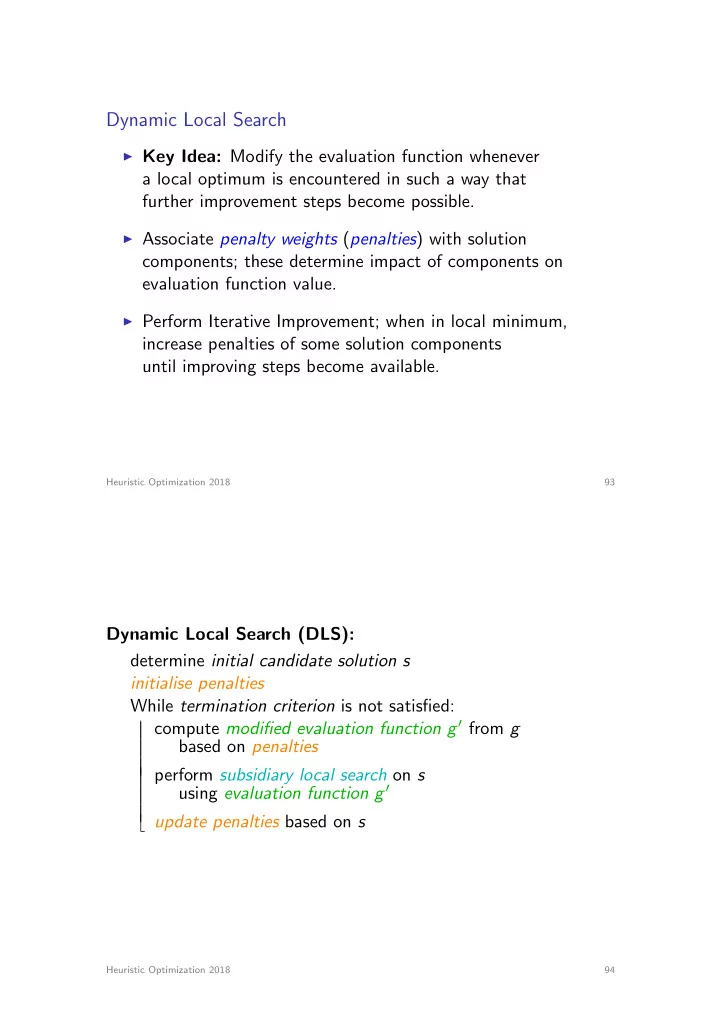
Dynamic Local Search I Key Idea: Modify the evaluation function whenever a local optimum is encountered in such a way that further improvement steps become possible. I Associate penalty weights ( penalties ) with solution components; these determine impact of components on evaluation function value. I Perform Iterative Improvement; when in local minimum, increase penalties of some solution components until improving steps become available. Heuristic Optimization 2018 93 Dynamic Local Search (DLS): determine initial candidate solution s initialise penalties While termination criterion is not satisfied: | compute modified evaluation function g 0 from g | | based on penalties | | | | | perform subsidiary local search on s | using evaluation function g 0 | | | b update penalties based on s Heuristic Optimization 2018 94

Dynamic Local Search (continued) I Modified evaluation function: g 0 ( π , s ) := g ( π , s ) + P i 2 SC ( π 0 , s ) penalty ( i ) , where SC ( π 0 , s ) = set of solution components of problem instance π 0 used in candidate solution s . I Penalty initialisation: For all i : penalty ( i ) := 0. I Penalty update in local minimum s : Typically involves penalty increase of some or all solution components of s ; often also occasional penalty decrease or penalty smoothing . I Subsidiary local search: Often Iterative Improvement . Heuristic Optimization 2018 95 Potential problem: Solution components required for (optimal) solution may also be present in many local minima. Possible solutions: A: Occasional decreases/smoothing of penalties. B: Only increase penalties of solution components that are least likely to occur in (optimal) solutions. Implementation of B (Guided local search): [Voudouris and Tsang, 1995] Only increase penalties of solution components i with maximal utility: f i ( π , s 0 ) util ( s 0 , i ) := 1 + penalty ( i ) where f i ( π , s 0 ) = solution quality contribution of i in s 0 . Heuristic Optimization 2018 96

Example: Guided Local Search (GLS) for the TSP [Voudouris and Tsang 1995; 1999] I Given: TSP instance G I Search space: Hamiltonian cycles in G with n vertices; use standard 2-exchange neighbourhood; solution components = edges of G ; f ( G , p ) := w ( p ); f e ( G , p ) := w ( e ); I Penalty initialisation: Set all edge penalties to zero. I Subsidiary local search: Iterative First Improvement. I Penalty update: Increment penalties for all edges with maximal utility by λ := 0 . 3 · w ( s 2-opt ) n where s 2-opt = 2-optimal tour. Heuristic Optimization 2018 97 Related methods: I Breakout Method [Morris, 1993] I GENET [Davenport et al. , 1994] I Clause weighting methods for SAT [Selman and Kautz, 1993; Cha and Iwama, 1996; Frank, 1997] I several long-term memory schemes of tabu search Dynamic local search algorithms are state of the art for several problems, including: I SAT, MAX-SAT I MAX-CLIQUE [Pullan et al. , 2006] Heuristic Optimization 2018 98

Hybrid SLS Methods Combination of ‘simple’ SLS methods often yields substantial performance improvements. Simple examples: I Commonly used restart mechanisms can be seen as hybridisations with Uninformed Random Picking I Iterative Improvement + Uninformed Random Walk = Randomised Iterative Improvement Heuristic Optimization 2018 99 Iterated Local Search Key Idea: Use two types of SLS steps: I subsidiary local search steps for reaching local optima as e ffi ciently as possible (intensification) I perturbation steps for e ff ectively escaping from local optima (diversification). Also: Use acceptance criterion to control diversification vs intensification behaviour. Heuristic Optimization 2018 100

Iterated Local Search (ILS): determine initial candidate solution s perform subsidiary local search on s While termination criterion is not satisfied: | | r := s | | perform perturbation on s | | perform subsidiary local search on s | | | | based on acceptance criterion , b keep s or revert to s := r Heuristic Optimization 2018 101 Note: I Subsidiary local search results in a local minimum. I ILS trajectories can be seen as walks in the space of local minima of the given evaluation function. I Perturbation phase and acceptance criterion may use aspects of search history ( i.e. , limited memory). I In a high-performance ILS algorithm, subsidiary local search , perturbation mechanism and acceptance criterion need to complement each other well. In what follows: A closer look at ILS Heuristic Optimization 2018 102

ILS — algorithmic outline procedure Iterated Local Search s 0 GenerateInitialSolution s ⇤ LocalSearch( s 0 ) repeat s 0 Perturbation( s ⇤ , history) s ⇤0 LocalSearch( s 0 ) s ⇤ AcceptanceCriterion( s ⇤ , s ⇤0 , history) until termination condition met end Heuristic Optimization 2018 103 basic version of ILS I initial solution: random or construction heuristic I subsidiary local search: often readily available I perturbation: random moves in higher order neighborhoods I acceptance criterion: force cost to decrease such a version of ILS .. I often leads to very good performance I only requires few lines of additional code to existing local search algorithm I state-of-the-art results with further optimizations Heuristic Optimization 2018 104

basic ILS algorithm for TSP I GenerateInitialSolution: greedy heuristic I LocalSearch: 2-opt, 3-opt, LK, (whatever available) I Perturbation: double-bridge move (a specific 4-opt move) I AcceptanceCriterion: accept s ⇤0 only if f ( s ⇤0 )  f ( s ⇤ ) Heuristic Optimization 2018 105 basic ILS algorithm for SMTWTP I GenerateInitialSolution: random initial solution or by EDD heuristic I LocalSearch: piped VND using local searches based on interchange and insert neighborhoods I Perturbation: random k -opt move, k > 2 I AcceptanceCriterion: accept s ⇤0 only if f ( s ⇤0 )  f ( s ⇤ ) Heuristic Optimization 2018 106

Quadratic Assignment Problem (QAP) I given: matrix of inter–location distances; d ij : distance from location i to location j I given: matrix of flows between objects; f rs : flow from object r to object s I objective : find an assignment (represented as a permutation) of the n objects to the n locations that minimizes n n X X min d ij f π ( i ) π ( j ) π 2 Π ( n ) i =1 j =1 π ( i ) gives object at location i I interest: among most di ffi cult combinatorial optimization problems for exact methods Heuristic Optimization 2018 107 basic ILS algorithm for QAP I GenerateInitialSolution: random initial solution I LocalSearch: iterative improvement in 2-exchange neighborhood I Perturbation: random k -opt move, k > 2 I AcceptanceCriterion: accept s ⇤0 only if f ( s ⇤0 )  f ( s ⇤ ) Heuristic Optimization 2018 108

basic ILS algorithm for SAT I GenerateInitialSolution: random initial solution I LocalSearch: short tabu search runs based on 1-flip neighborhood I Perturbation: random k -flip move, k >> 2 I AcceptanceCriterion: accept s ⇤0 only if f ( s ⇤0 )  f ( s ⇤ ) Heuristic Optimization 2018 109 ILS is a modular approach Performance improvement by optimization of modules I consider di ff erent implementation possibilities for modules I fine-tune modules step-by-step I optimize single modules without considering interactions among modules local optimization of ILS Heuristic Optimization 2018 110

ILS — initial solution I determines starting point s ⇤ 0 of walk in S ⇤ I random vs. greedy initial solution I greedy initial solutions appear to be recomendable I for long runs dependence on s ⇤ 0 should be very low Heuristic Optimization 2018 111 ILS for FSP, initial solution 3880 Greedy start Random start 3860 3840 3820 Makespan 3800 3780 3760 3740 3720 1 10 100 1000 10000 CPU time [sec] Heuristic Optimization 2018 112

ILS — perturbation I important: strength of perturbation I too strong : close to random restart I too weak : LocalSearch may undo perturbation easily I random perturbations are simplest but not necessarily best I perturbation should be complementary to LocalSearch Heuristic Optimization 2018 113 double-bridge move for TSP I small perturbation good also for very large-size TSP instances I complementary to most implementations of LK local search I low cost increase C B Old: A-B-C-D New: A-D-C-B D A Heuristic Optimization 2018 114

sometimes large perturbations needed I example: basic ILS for QAP given is average deviation from best-known solutions for di ff erent sizes of the perturbation (from 3 to n ); averages over 10 trials; 60 seconds on a 500MHz Pentium III. instance 3 n / 12 n / 6 n / 4 n / 3 n / 2 3 n / 4 n 2.51 2.51 2.04 1.06 0.83 0.42 0.0 0.77 kra30a 0.65 1.04 0.50 0.37 0.29 0.29 0.82 0.93 sko64 2.31 2.24 1.91 1.71 1.86 2.94 3.13 3.18 tai60a 2.44 0.97 0.67 0.96 0.82 0.50 0.14 0.43 tai60b Heuristic Optimization 2018 115 Adaptive perturbations I single perturbation size not necessarily optimal I perturbation size may vary at run-time; done in basic Variable Neighborhood Search I perturbation size may be adapted at run-time; leads to reactive search Complex perturbation schemes I optimizations of subproblems [Louren¸ co, 1995] I input data modifications I modify data definition of instance I on modified instance run LocalSearch using input s ⇤ , output is perturbed solution s 0 Heuristic Optimization 2018 116