DurableGoods Monopoly with Varying Demand Simon Board Department - PDF document

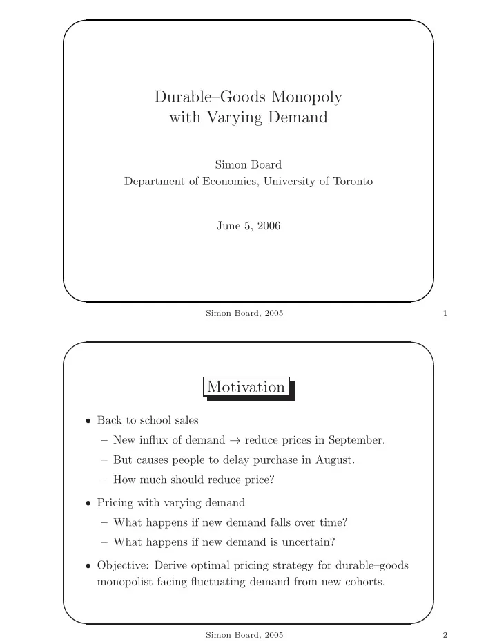
✬ ✩ Durable–Goods Monopoly with Varying Demand Simon Board Department of Economics, University of Toronto June 5, 2006 ✫ ✪ Simon Board, 2005 1 ✬ ✩ Motivation • Back to school sales – New influx of demand → reduce prices in September. – But causes people to delay purchase in August. – How much should reduce price? • Pricing with varying demand – What happens if new demand falls over time? – What happens if new demand is uncertain? • Objective: Derive optimal pricing strategy for durable–goods monopolist facing fluctuating demand from new cohorts. ✫ ✪ Simon Board, 2005 2

✬ ✩ Durable Goods Monopoly • No new entry of consumers (Stokey, 1979) – Consumers enter market in period 1. – Firm choose prices { p 1 , . . . , p T } . – Agents choose when to buy. – Solution: charge static monopoly price forever. • Identical entry each period (Conlisk et al, 1984) – Solution: charge static monopoly price forever. ✫ ✪ Simon Board, 2005 3 ✬ ✩ Varying Demand • What if new demand varies over time? – Theory of dynamic pricing. – Scope for intertemporal price discrimination. • Technique – Method to solve dynamic mechanism design problems. – Simple marginal revenue interpretation. • Fast rises and slow falls – Demand growing = ⇒ price increases quickly. – Demand dying = ⇒ price decreases slowly. • Application: propagation of demand cycles. – Prices exceed the average–demand price. ✫ ✪ – The lowest price is at last period of the “slump”. Simon Board, 2005 4

✬ ✩ The Model • Time is discrete, t ∈ { 1 , . . . , T } , where allow T = ∞ . – Consumers’ and firm’s information represented by filtered space (Ω , F , {F t } , Q ). – Common time– t discount rate, δ t ∈ ( ǫ, 1 − ǫ ), is F t –adapted. – Total discount factor ∆ t := � t i =1 δ s . • Consider consumer with value θ ∈ [ θ, θ ] – If buy at time t and price p t get ( θ − p t )∆ t . – If do not purchase get zero. • Each period consumers of measure f t ( θ ) enter market – Distribution function F t ( θ ), survival function F t ( θ ). – Total measure F t ( θ ). – New demand, f t ( θ ), is F t –adapted. ✫ ✪ The Model 5 ✬ ✩ Payoffs • Consumer’s Problem – Consider consumer ( θ, t ) with value θ who enters at time t . – Given sequence of F t –adapted prices { p 1 , . . . , p T } . – Choose purchasing time τ ( θ, t ) to maximise expected utility. u t ( θ ) = E [( θ − p τ )∆ τ ] • Firm’s Problem – Assume marginal cost is zero. – Choose F t –adapted prices { p t } to maximise expected profit � T � θ � � Π = E ∆ τ ∗ ( θ,t ) p τ ∗ ( θ,t ) dF t θ t =1 where τ ∗ ( θ, t ) maximises the consumer’s utility, u t ( θ ). ✫ ✪ • Notable assumptions: No resale. Firm commits to prices. The Model 6

✬ ✩ Consumer Surplus and Welfare • Purchase time optimal so use envelope theorem, �� θ � u t ( θ ) = E ∆ τ ∗ ( x,t ) dx + u ( θ, t ) θ using Milgrom–Segal (2002) since space of stopping times complex. • Consumer surplus from generation t , � θ �� θ � u t ( θ ) dF t = E ∆ τ ∗ ( θ,t ) F t ( θ ) dθ θ θ • Welfare from generation t , �� θ � W t = E θ ∆ τ ∗ ( θ,t ) dF t θ ✫ ✪ Costs are zero so the welfare is maximised by setting p t = 0. Solution Technique 7 ✬ ✩ Firm’s Problem • Define marginal revenue with respect to price as m t ( θ ) := θf t ( θ ) − F t ( θ ) • Expected profit is welfare minus consumer surplus, � T � θ � � Π = E ∆ τ ∗ ( θ,t ) m t ( θ ) dθ θ t =1 • Profit is discounted sum of marginal revenues. • Marginal revenue sticks to each agent ( θ, t ). • The firm’s problem is to chooses prices { p 1 , . . . , p T } to maximise Π subject to τ ∗ ( θ, t ) maximising u t ( θ ). ✫ ✪ Solution Technique 8

✬ ✩ Consumer’s Problem and Cutoffs Lemma 1. The earliest purchasing rule, τ ∗ ( θ, t ) , obeys: [ existence ] τ ∗ ( θ, t ) exists. [ θ –monotonicity ] τ ∗ ( θ, t ) is decreasing in θ . [ non–discrimination ] τ ∗ ( θ, t L ) ≥ t H = ⇒ τ ∗ ( θ, t L ) = τ ∗ ( θ, t H ) , for t H ≥ t L . • Characterise τ ∗ ( θ, t ) by F t –adapted cutoffs θ ∗ t := inf { θ : τ ∗ ( θ, t ) = t } • Back out prices from cutoffs: ( θ ∗ t − p ∗ τ ≥ t +1 E [( θ ∗ t − p ∗ t )∆ t = max τ )∆ τ ] ✫ ✪ Solution Technique 9 ✬ ✩ General Solution Definition. Cumulative marginal revenue equals M 1 ( θ ) := m 1 ( θ ) and M t ( θ ) := m t ( θ ) + min { M t − 1 ( θ ) , 0 } . Assumption (MON). M t ( θ ) is quasi–increasing ( ∀ t ). t = M − 1 Theorem 1. Under (MON) the optimal cutoffs are θ ∗ (0) . t • Period t = 1 – Sell to agent θ iff m 1 ( θ ) ≥ 0 • Period t = 2 – Form cumulative MR, M 2 ( θ ) = m 2 ( θ ) + min { M t − 1 ( θ ) , 0 } – Sell to agent θ iff M 2 ( θ ) ≥ 0 • Cutoffs are determined by past demand. ✫ • Prices are determined by future cutoffs. ✪ Optimal Pricing 10

✬ ✩ (1) Monotone Deterministic Demand • Suppose demand deterministic. Proposition 2a. Suppose demand is increasing, m − 1 t +1 (0) ≥ m − 1 t (0) . t = m − 1 t = m − 1 Then θ ∗ t (0) and prices are p ∗ t (0) . Proposition 2b. Suppose demand is decreasing, m − 1 t +1 (0) ≤ m − 1 t (0) . t = m − 1 Then θ ∗ ≤ t (0) and prices are T �� ∆ s � � � − ∆ s +1 � m − 1 p ∗ � t = E ≤ s (0) � F t � ∆ t ∆ t s = t := m − 1 • Myopic price: p M t (0). t t := m − 1 • Average–Demand price: p A ≤ T (0) ✫ ✪ Applications 11 ✬ ✩ (2) Deterministic Cycles • Suppose demand follows K repetitions of { f 1 ( θ ) , . . . , f T ( θ ) } Proposition 4. For k ≥ 2 , cycles are stationary. Proposition 5. For k ≥ 2 , optimal prices always lie above the average–demand price, m − 1 ≤ T (0) . • Price discrimination bad for all customers. Proposition 6. For k ≥ 2 , if cycles are simple the price is lowest at the end of the slump. ✫ ✪ Applications 12

✬ ✩ (3) IID Demand • Demand drawn from { m i ( θ ) } with prob { q i } . – Average marginal revenue m A ( θ ) = � i q i m i ( θ ) . – Average–demand price p A := [ m A ] − 1 (0) . t ≥ p A and Proposition 7. The SLLN implies lim t →∞ θ ∗ t ≥ p A a.s.. lim t →∞ p ∗ • Stochastic equivalent of Proposition 5 (i.e. with deterministic cycles, prices exceed the average–demand price). ✫ ✪ Applications 13 ✬ ✩ Summary • Derived optimal pricing strategy for durable–goods monopolist facing varying demand. • Award good to agents with positive cumulative MR. • Prices rise quickly and fall slowly. • Asymmetry pushes prices upwards. ✫ ✪ The End 14