[PDF] - Part I: Exercise of Monopoly Power Chapter 1: Monopoly Two PDF Document

SLIDE 1

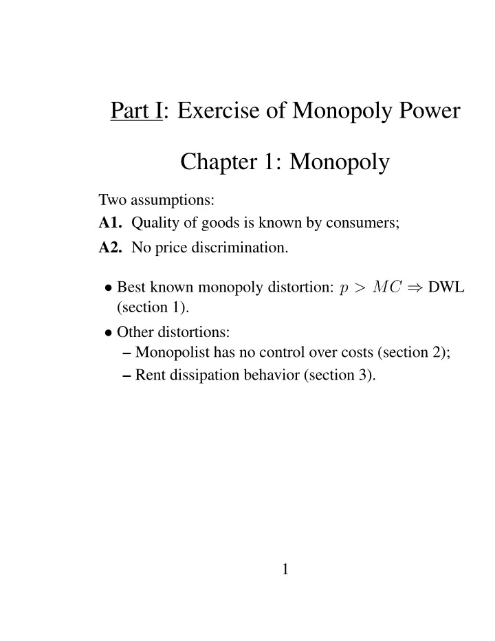
Part I: Exercise of Monopoly Power Chapter 1: Monopoly

Two assumptions:

A1. Quality of goods is known by consumers;
A2. No price discrimination.
Best known monopoly distortion: p > MC ⇒ DWL

(section 1).

Other distortions:

– Monopolist has no control over costs (section 2); – Rent dissipation behavior (section 3). 1

SLIDE 2

1 Pricing Behavior

Distortion associated to monopolist pricing.

1.1 A Single-Product Monopolist

q = D(p) demand function, D0(p) < 0, p = P(q) the

inverse demand function.

C(q) the cost of producing q units of good, C0(q) > 0.
Elasticity of Demand:

ε = −D0(p) D(p) p

Program of the monopoly (in quantity)

max

q

{qP(q) − C(q)}

FOC: qP 0(q) + P(q) − C0(q) = 0

⇒ qm

SOC: qP 00(q) + 2P 0(q) − C00(q) < 0 Result 1: MR(qm) = MC(qm) ⇒ pm > MC 2

SLIDE 3

Program of the monopoly (in price)

max

p

{pD(p) − C(D(p))}

FOC : pD0(p) + D(p) − C0(D(p))D0(p) = 0 ⇒ pm SOC :

pD00(p) + 2D0(p) − C00(D(p))(D0(p))2 − C0(D(p))D00(p) <

+ assumptions on D00(p) and C00(q) (concavity or quasi

concavity). Result 2:

$ ≡ pm − C0(.) pm = 1 ε

where $ is the Lerner index or relative markup. Example Demand function q = kp−ε where k > 0. Result 3: Monopolist always operates where ε > 1.

See graph
Formally:

pm−C0(.) pm

< 1 because pm − C0(.) < pm so, 1 ε < 1 ⇒ ε > 1

Result 4: Monopoly price is a non decreasing function

f marginal cost.

3

SLIDE 4

Proof:

2 alternative cost functions C1(.) and C2(.).
C0

2(q) > C0 1(q) for any q.

pm

1 , qm 1 if C1(.), and pm 2 , qm 2 if C2(.).

If cost is C1(.) (resp. C2(.)), pm

1 (resp. pm 2 ) is charged

by the monopolist

pm

1 qm 1 − C1(qm 1 ) ≥ pm 2 qm 2 − C1(qm 2 )

pm

2 qm 2 − C2(qm 2 ) ≥ pm 1 qm 1 − C2(qm 1 )

Sum these 2 inequalities

C2(qm

1 ) − C2(qm 2 ) ≥ C1(qm 1 ) − C1(qm 2 )

C2(qm

1 ) − C1(qm 1 ) − [C2(qm 2 ) − C1(qm 2 )] ≥ 0

R qm

1

qm

2 [C0

2(x) − C0 1(x)] dx ≥ 0

Because C0

2(x) > C0 1(x) then qm 1 ≥ qm 2 and pm 1 ≤ pm 2 .

Appropriate measure of distortion is the loss of social

welfare: the dead-weight loss.

see graph

4

SLIDE 5

Benchmark case: perfect competition

Result 5: The welfare loss does not necessarily decrease with the elasticity of demand, even though the relative markup does. Proof: exercise 1.1. page 67 Tirole.

DWL determines the loss from a monopoly to an

idealistic situation.

DWL is one distortion created by a monopoly power.
What kind of public intervention?
Example: commodity taxation. Policy to restore social
ptimum.
Government imposes a tax on the output, t.
The program of the monopolist becomes:

max

p

{pD(p + t) − C(D(p + t))} FOC : pD0(p + t) + D(p + t) − C0(D(q + t))D0(p + t) = ⇔ [D(p + t) − tD0(p + t)] +D0(p + t) [p + t − C0(D(q + t))] = 0

From the second term: p + t = C0(.).

5

SLIDE 6

First term:

D(p + t) = tD0(p + t) ⇒ t = D(pc)

D0(pc)

and thus t < 0 = subsidy!
Why?

– monopoly price induces consumers to consume too little. – If subsidy, consumption will increase.

But the government needs to have information con-

cerning cost and demand. – Demand can be found with statistic studies. – Difficult to get information on costs.

Incentive theory.

6

SLIDE 7

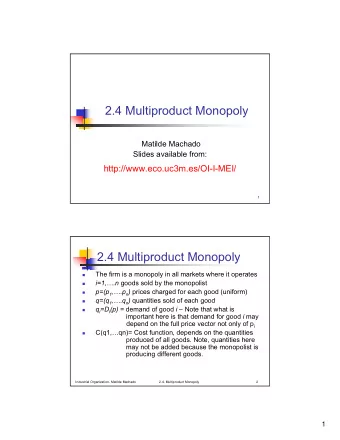
1.2 Multi-Product Monopolist

Multi-product firm has a monopoly power over all

goods.

qi = Di(p), demand for good i = 1, ...., n.
Prices, p = (p1, p2, ...., pn).
Quantities q = (q1, q2, ..., qn).
Cost C(q1, q2, ..., qn).
Single-product firm (n pricing problems) ⇔ multi-

product firm with – independent demands: qi = Di(pi) – separable costs: C(q1, q2, ..., qn) = Pn

i=1 Ci(qi).

For each good i

$i = pm

i − C0 i

pm

i

= 1 εi

Result 6: The markup is higher on goods with a lower elasticity of demand (Ramsey pricing). 7

SLIDE 8

General multi-product monopolist program is

max

p1,p2,....,pn

( n X

i=1

piDi(p) − C(D1(p), D2(p), ..., Dn(p)) )

FOCi : pi

∂Di(p) ∂pi

+ Di(p) + X

j6=i

pj

∂Dj(p) ∂pi

−

n

X

k=1 ∂C(.) ∂qk ∂Dk(p) ∂pk

∀i, ∀k 6= i

SOC must be satisfied.

2 polar cases:

1. dependent demands, separable costs;
2. independent demands, dependent costs.

1.2.1 Dependent demands and separable costs

Example: set of divisions
qi = Di(p)
C(q1, q2, ..., qn) = Pn

i=1 Ci(qi)

Program of the multi-product monopolist is

8

SLIDE 9

max

p1,p2,....,pn

( n X

i=1

piDi(p) −

n

X

i=1

Ci(Di(p)) )

from (1)

⇒ pi − ∂Ci(.)

∂qi

pi = − Di(p) + P

j6=i ∂Dj(p) ∂pi (pj − ∂Cj(.) ∂qj )

pi

∂Di(p) ∂pi

Own elasticity of demand

εii = − pi Di(p) ∂Di(p) ∂pi

Cross elasticity of demand for good j

εij = − pi Dj(p) ∂Dj(p) ∂pi

FOC becomes

pi − ∂Ci(.)

∂qi

pi = 1 εii − X

j6=i

³ pj − ∂Cj(.)

∂qj

´ Dj(p)εij εiipiDi(p)

Sign of the second term? (depends on the sign of εij)

9

SLIDE 10

– If (−), $i >

1 εii, and thus higher price than in the

case of a single-product monopolist. – if (+), $i < 1

εii, and thus lower price.

If goods are substitutes, ∂Dj(p)

∂pi

> 0 for j 6= i so εij < 0.

– thus $i > 1

εii ⇒ pi > pm.

If goods are complements, ∂Dj(p)

∂pi

< 0 for j 6= i so εij > 0

– thus $i < 1

εii ⇒ pi < pm.

Example: Intertemporal pricing.
Single-product monopolist
2 periods: t = 1, t = 2.
At t = 1,

– demand function q1 = D1(p1) – cost function C(q1)

At t = 2,

– demand function q2 = D2(p2, p1) – cost function C(q2)

Goodwill effect: ∂D2(.)

∂p1

< 0

10

SLIDE 11

Monopolist’s profit

p1D1(p1) − C(q1) + δ[p2D2(p2, p1) − C(D2(p2, p1))]

where δ is the discount factor.

⇔ multi-product firm with interdependent demands.

FOC1 : p1

∂D1 ∂p1 + D1(.) − ∂C(.) ∂q1 ∂D1 ∂p1 + δ(p2 − ∂C(.) ∂q2 )∂D2 ∂p1 = 0

FOC2 : p2

∂D2 ∂p2 + D2(p2, p1) − ∂C(.) ∂q2 ∂D2 ∂p2 = 0

In the second period, monopoly price as

$2 = 1 ε22 ⇒ pm

2

In the first period, the monopolist sets a lower price as

$1 < 1 ε11 ⇒ p1 < pm

1

Thus, the monopolist reduces the price at date 1

(sacrifice some short run profit) to increase the demand (and thus the profit) at date 2. 11

SLIDE 12

1.2.2 Independent demands and dependent costs

The demand functions are independent, qi = Di(pi).
C(q1, q2, ..., qn)
The program is

max

p1,p2,....,pn

( n X

i=1

piDi(pi) − C(q1, q2, ..., qn) )

Example: learning-by-doing
Cost reduction can be achieved over time simply

because of learning.

Example: semi-conductor industry, computers industry
Single-Product monopolist
2 periods: t = 1, t = 2.
At t = 1,

– demand function q1 = D1(p1) – cost function C1(q1)

At t = 2,

– demand function q2 = D2(p2) – cost function C2(q2, q1) with ∂C2(.)

∂q1

< 0

12

SLIDE 13

Monopolist’s profit

p1D1(p1)−C1(D1(p1))+δ[p2D2(p2)−C2(D2(p2), D1(p1))]

where δ is the discount factor.

FOC1 : p1

∂D1 ∂p1 + D1(p1) − ∂C1(.) ∂q1 ∂D1 ∂p1 − δ∂C2(.) ∂q1 ∂D1 ∂p1 = 0

FOC2 : p2

∂D2 ∂p2 + D2(p2) − ∂C2(.) ∂q2 ∂D2 ∂p2 = 0

In the second period, monopoly price as

$2 = 1 ε22

In the first period, the monopolist sets a lower price as

$1 < 1 ε11

Thus, the monopolist reduces the price at date 1 (and

sells more in the 1st period) to reduce the cost (and thus increase the profit) in the 2d period. 13

SLIDE 14

However, in a more general setting (exercise 1.7) where

the output grows over time with stationary demand and the cost decreases with experience, there are 2 effects:

a. myopic behavior: as MC decreases, quantity must

increase.

b. non myopic behavior: higher quantity at the

beginning.

⇒First effect dominates the second effect: The

monopolist does not reduce the price in the first period. 14

SLIDE 15

2 Cost Distortion

Distortion on the supply side.
For given quantities, a monopolist may produce at a

higher cost than would a competitive firm.

Delegation problem

– shareholders and manager do not have the same

bjective.

– Thus, problem of monitoring and controlling. – ⇒ inefficiency.

How this inefficiency is affected by market power?
Shareholders can use yardstick competition (compar-

ison with other firms)

Example: Ford management can be compared to GM.
But you need to have another firm to be able to

compare!

These extra costs add to the DWL.

15

SLIDE 16

3 Rent Seeking behavior

Third kind of distortion: the wasteful expenses incurred

by a firm to get and to maintain a monopoly position.

The rent of the monopolist (profit) may lead to

rent-seeking behavior. – Firms will tend to spend money and effort to acquire the monopoly position; – Once installed they will tend to keep on spending money and exerting effort to maintain it.

Different kinds of expenses:

– Strategic expenses

∗ R&D cost of obtaining a patent (chapter 10), ∗ accumulation of capital, ∗ barriers to entry (chapter 8).

– Administrative expenses

∗ cost of lobbying, ∗ advertising campaigns, ∗ legal expenses against charges of antitrust

violation. 16

SLIDE 17

Axiom (Porter, 75) says that
1. rent dissipation (total expenses to obtain rent = amount
f the rent). This is the zero-profit free entry condition.
2. socially wasteful dissipation: it is not socially valuable.

Regulated monopoly is allocated on the basis of lobbying influence.

So, rent-seeking behavior certainly wastes some of the

monopoly profit.

The monopoly profit may be part of the welfare loss,

but what fraction, it is not clear... 17

SLIDE 18

4 Conclusion

Distortions created by monopoly power

1. high prices, DWL
2. inefficiency (because objectives of managers are

different to those of the owner of the firm)

3. dissipation of the monopoly profit.

But a monopoly can have some advantages:

1. under increasing return to scale, production by a single

firm is technologically more efficient (it is less costly to have only one firm, natural monopoly). It prevents a wasteful duplication of fixed costs.

2. Schumpeter said that monopoly may be a necessary