Drivetrain Innovations BV - - PDF document

SLIDE 1

Proceeding zyxwvutsrqponmlkjihgfedcbaZYXWVUTSRQPONMLKJIHGFEDCBA

• f the 2004 American Control Conference
• Boston. Massachusetts June 30 -July

2,2004

FrA05.6 zyxwvutsrqponmlkjihgfedcbaZYXWVUTSRQPONMLKJIHGFEDCBA

Simulation and

Alex Serrarens

Drivetrain Innovations BV zyxwvutsrqponmlkjihgfedcbaZYXWVUTSRQPONMLKJIHGFEDCBA

serrarens@dtinnovations.nl

Control of an Automotive Dry Clutch

Marc Dassen Maarten Steinbuch

Control Systems Technology

Technische Universiteit Eindhoven Faculty of Mechanical Engineering

Control Systems Technology

m.h.m.dassen@student.tue.nl

m.steinbuch@tue.nl

P.O. Box 513, 5600 MB Eindhoven, The Netherlands

www.aes.wtb.tue.nl zyxwvutsrqponmlkjihgfedcbaZYXWVUTSRQPONMLKJIHGFEDCBA

Absmacf-In this paper the dynamic behavior and control

• f an automotive dry clutch is analyzed. Thereto, a straight-

forward model of the clutch is embedded within a dynamic model of an automotive powertrain comprising an internal combustion engine, drivetrain and wheels moving a vehicle through tire-road adhesion. The engagement of the clutch is illustrated using the model best suited for simulation, based

• n work of Karnopp. These simulation results are used for

conceiving a decoupling controller for the engine and clutch

• torque. Simulation results with the controller show significant

improvement over the un-controlled case in terms of vehicle launch comfort. A modified controller is proposed that results in even more appreciated drive comfort while not deteriorating

• ther system behavior.
• I. INTRODUCTION

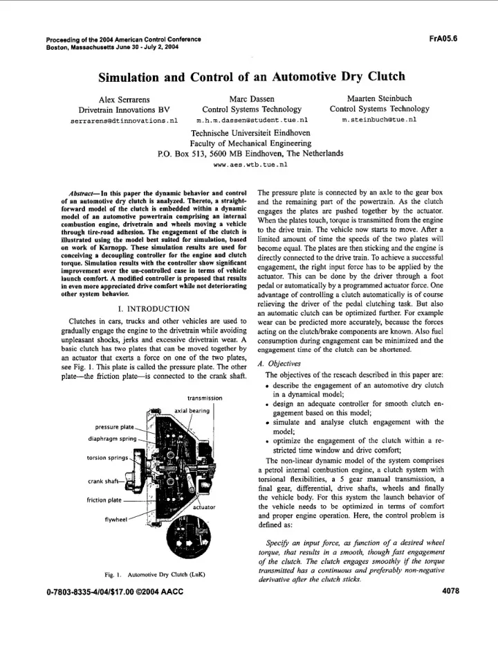
Clutches in cars, trucks and other vehicles are used to gradually engage the engine to the drivetrain while avoiding unpleasant shocks, jerks and excessive drivetrain wear. A basic clutch has two plates that can he moved together by an actuator that exerts a force on one of the two plates, see Fig. 1. This plate is called the pressure plate. The other plate-the friction p l a t e i s connected to the crank shah. transmission axial Pearing zyxwvutsrqponmlkjihgfedcbaZYXWVUTSRQPONMLKJIHGFEDCBA

I

pressure pla

diaphragm rpri torslo" rprmgr

crank s h a h friction plate ~

flywheel'

• Fig. 1.

0-7803-8335-4104/$17.00 02004 AACC

Automotive Dry Clutch (LuK)

The pressure plate is connected by an axle to the gear box and the remaining part of the powertrain. As the clutch engages the plates are pushed together by the actuator. When the plates touch, torque is transmitted from the engine to the drive train. The vehicle now starts to move. After a limited amount of time the speeds of the two plates will become equal. The plates are then sticking and the engine is directly connected to the drive train. To achieve a successful engagement, the right input force has to be applied by the

• actuator. This can be done by the driver through a foot

pedal or automatically by a programmed actuator force. One advantage of controlling a clutch automatically is of course relieving the driver of the pedal clutching task. But also an automatic clutch can be optimized further. For example wear can be predicted more accurately, because the forces acting on the clutchibrake components are known. Also fuel consumption during engagement can be minimized and the engagement time of the clutch can he shortened.

A . Objectives

The objectives of the reseach described in this paper are: describe the engagement of an automotive zyxwvutsrqponmlkjihgfedcbaZYXWVUTSRQPONMLKJIHGFEDCBA

dry clutch

in a dynamical model;

.

design an adequate controller for smooth clutch en- gagement based on this model; simulate and analyse clutch engagement with the model;

.

• ptimize the engagement of the clutch within a re-

stricted time window and drive comfort; The non-linear dynamic model of the system comprises a petrol intemal combustion engine, a clutch system with torsional flexibilities, a zyxwvutsrqponmlkjihgfedcbaZYXWVUTSRQPONMLKJIHGFEDCBA

5 gear manual transmission, a

final gear, differential, drive shafts, wheels and finally the vehicle body. For this system the launch behavior of the vehicle needs to be optimized in terms of comfort and proper engine operation. Here, the control problem is defined as: Specify an input force, as function of a desired wheel torque, that results zyxwvutsrqponmlkjihgfedcbaZYXWVUTSRQPONMLKJIHGFEDCBA

i n a smooth, though fast engagement

• f the clutch. The clutch engages smoothly if the torque

transmitted has a continuous and preferably non-negative derivafive aBer the clutch sfickr.

4078

SLIDE 2 engine clutch vehicle zyxwvutsrqponmlkjihgfedcbaZYXWVUTSRQPONMLKJIHGFEDCBA

• Fig. zyxwvutsrqponmlkjihgfedcbaZYXWVUTSRQPONMLKJIHGFEDCBA
• 2. PoweNain model

O u r zyxwvutsrqponmlkjihgfedcbaZYXWVUTSRQPONMLKJIHGFEDCBA

main contributions to existing work comprises an

• verview of different modelling st”ctures and a modifica-

tion of a known decoupliug technique into a controller that enables direct control over a drive comfort variable. zyxwvutsrqponmlkjihgfedcbaZYXWVUTSRQPONMLKJIHGFEDCBA

• B. Outline

The remainder of the paper is organized as follows. In section zyxwvutsrqponmlkjihgfedcbaZYXWVUTSRQPONMLKJIHGFEDCBA

1 1 , the powertrain system under consideration is pre-

sented and literature that covers either modelling or control issues of this type of system is cited. Section I11 presents three modelling techniques for the non-linear model. One of these models is preferred for simulation and analysis. Using the preferred model, in section IV the system is simulated using open loop commands. The results are analyzed and a decoupling control structure is proposed for the zyxwvutsrqponmlkjihgfedcbaZYXWVUTSRQPONMLKJIHGFEDCBA

two

control inputs, i.e. engine torque and clutch torque. With this decoupling controller simulations are carried out and parameters are tuned for optimal behavior. Furthermore, the modified control structure is proposed. The improvements in drive comfort are again illustrated through simulations.

• 11. PASSENGER

CAR POWERTRAIN SUBSYSTEMS Passenger car powertrains comprise the ensemble of the internal combustion engine, launch device, transmission system, differential and the drive shah. For modelling purposes we need to extend this definition with the wheels, tires and vehicle, see Fig. 2. In case of (automated) manual transmissions the launch device is mostly a zyxwvutsrqponmlkjihgfedcbaZYXWVUTSRQPONMLKJIHGFEDCBA

dry clutch, whereas for automatic and

continuously variable transmission this may be either an

• il immersed (wet) clutch or hydraulic torque converter. In

this paper we only consider a powertrain equipped with manual transmission and automated dry clutch assembly. In the next subsections, the various elements of the powertrain are briefly discussed and basic equations for them are

• given. In section III, these equations are assembled in

three different ways towards a total powertrain model. In this powertrain model inertias, are appropriately taken into

• account. Furthermore, we follow some of the modelling

principles proposed in [I] and [2]. For the modelling of the clutch we exploit the work presented in [3]. Within the scope of this paper, the transmission and engine need no fmther detailing other than first principle modelling.

• A. engine

The engine torque zyxwvutsrqponmlkjihgfedcbaZYXWVUTSRQPONMLKJIHGFEDCBA T, is assumed to have infinitely fast dynamics and is only restricted by an lower and upper

• bound. Here, the upper hound is a quadratic function of

the engine speed zyxwvutsrqponmlkjihgfedcbaZYXWVUTSRQPONMLKJIHGFEDCBA

U&, whereas the lower bound equals zero.

Although this represents a rather crude approximation of the real engine torque it suffices for our analysis. The engine torque is described by:

• 5 r, 5 T,,-~.~o-~(w,,--w~), zyxwvutsrqponmlkjihgfedcbaZYXWVUTSRQPONMLKJIHGFEDCBA

(1) where T

, , , = 160 (”)

is the maximum engine torque achieved at w, =

q

• =

300 (rads). Also the engine speed is hounded, i.e.

U&& 5 w, 5 U&,,,

(2) where w

. , , = 100 (rads) and

=

600 (rad/s). The engine inertia& is driven by the engine torque and is loaded by the clutch torque T , . The equation of motion is then governed by: Je& = r,

• zyxwvutsrqponmlkjihgfedcbaZYXWVUTSRQPONMLKJIHGFEDCBA

z.

(3)

• B. clutch

The clutch system, shown in Fig. 1 exists of a housing, pressure plates, friction plates, a clutch disc with torsion “dampers” and a release mechanism. The clutch disk is shoved onto the transmission input shaft and is radially fixed by a splined interface. The clutch is normally closed as the diaphragm spring is pre-tensioned when assembled. The axial bearing can slide over the transmission input shaft and push against the fingers of the diaphragm spring. The direction of the release force is swapped through the lever joints and releases the pressure from the clutch disk which is then able to rotate independently from the engine. The clutch disc is equipped with torsional dampers which are in fact coil springs that connect various segments

• f the clutch disc. These springs aim at maximizing the

comfort level for the driver, when opening and closing the

• clutch. Due to the various springs in parallel and series

formation a sequence of piece-wise linear stiffness regions with hysteresis emerges. Here, we use a simplified model for this complex coil spring assembly. Furthermore, the clutch plate segments introduce (mandatory) damping due to friction between them. The clutch system is modelled as depicted in Fig. 2. The clutch disc has inertia J, and the transmission (see also section C) has inertia 4. The torque transmitted through the clutch (both in slipping and engaged state) is indicated by z. The speed of the clutch disc and transmission input shaft are presented by o, and y,

• respectively. We define

(pd =

f p c

• 9

and the nonlinear stiffness of the coil springs is k(%) is simplified into the form: 60 [Nm/rad] for - 0.25 5 (pd 5 0.35,

(4)

1000 [“/rad] else. 4079

SLIDE 3

I ) slipping clutch: zyxwvutsrqponmlkjihgfedcbaZYXWVUTSRQPONMLKJIHGFEDCBA

The differential equation governing the clutch dynamics can be expressed as: Jc& zyxwvutsrqponmlkjihgfedcbaZYXWVUTSRQPONMLKJIHGFEDCBA

= zyxwvutsrqponmlkjihgfedcbaZYXWVUTSRQPONMLKJIHGFEDCBA Tc

• zyxwvutsrqponmlkjihgfedcbaZYXWVUTSRQPONMLKJIHGFEDCBA

Td -

bc.

(q

• zyxwvutsrqponmlkjihgfedcbaZYXWVUTSRQPONMLKJIHGFEDCBA

a)

pd = zyxwvutsrqponmlkjihgfedcbaZYXWVUTSRQPONMLKJIHGFEDCBA

k(qd) ' (%

• a) zyxwvutsrqponmlkjihgfedcbaZYXWVUTSRQPONMLKJIHGFEDCBA

(5)

(6)

The torque through the clutch while slipping is given by:

C = Fn

P & sign(& -

4,

(7) in which p is the friction coefficient of the clutch surface material, R, is te active radius of the clutch plates and the normal actuation force on the clutch plate is given by F". 2) sticking clutch: When the clutch is sticking, the engine degree of freedom is rigidly coupled to the clutch disk at the friction interface. The two differential equations

• f the engine and the clutch, i.e. (3)

and (5) can he reduced to a single differential equation: (Je+Jc)hc

=

T, - - 6,. zyxwvutsrqponmlkjihgfedcbaZYXWVUTSRQPONMLKJIHGFEDCBA

(q

• a)

(8) The sticking of the clutch sustains as long as the torque transmitted through clutch (Tc) remains below the maxi- mally transmittable torque T , " , which is given by:

cm"

=

• F. bCict

R, sign(

T,) . zyxwvutsrqponmlkjihgfedcbaZYXWVUTSRQPONMLKJIHGFEDCBA

(9)

Here, we assume b.tick = 2 .

• p. Furthermore, the term

sign(T,) is non-positive in the case of vehicle (engine) braking and positive in all other cases.

• C. transmission & drive shops

The transmission is connected with its input shaft to the flexible friction plate of the clutch. The input shaft is connected through a gear mesh to the second shaft. The second shaft is connected via the final drive to the

• differential. The gear ratio selected within the transmission

is denoted by r, and the final drive gear ratio by rf. The

• verall transmission ratio r is then defined by:

where o f is the speed of the output gear of the final

• drive. We do not consider transmission gear shifting and

all rotating transmission parts are assumed to be lumped in one inertia 5 , damped by viscous damping b,. We assume straight line driving, hence the differential does not introduce a difference in speed of the left and right drive

• shaft. Therefore, the two drive shafts are lumped into one

stiffness ks. The model of the transmission can be presented as in Fig. 2. The equations of motion of the transmission model are given by:

Jtuj,

=

T d

• bt. - zyxwvutsrqponmlkjihgfedcbaZYXWVUTSRQPONMLKJIHGFEDCBA

(11)

p s =

ks(of- G)

(12)

D.

wheels & tyres The model structure in Fig. 2 we assume that the driving wheels and tyres are modelled as an inertia connected to the vehicle mass through a linear damper with coefficient b,. This damper forms the slipping traction interface between tyres and road. In literature, [l] a non-linear tyre traction model is proposed as a function of the tyre slip s: where w, is the wheel speed, R, is the dynamic wheel radius in (m) and vy is the vehicle speed in ( d s ) . Although a non-linear tyre slip model is available in literature [I], we prefer to use the linear approximation for it at low vehicle speeds. Finally, the tyres experience a rolling torque T

,

due to deformation of the tyre surface. The differential equation goveming the wheel and tyre dynamics is then given by: Jw& =

G

• b, .s-

aT,.

(14)

The inertia J, equals that of the hvo driving wheels. Furthermore, a is the fraction of the vehicle mass that rests upon the driving wheels.

• E. vehicle

The vehicle acceleration is the result of the traction torque, air drag and the rolling resistance of the driven wheels (rear wheels for front-wheel-drive cars), i.e.

(15)

V"

1 R w

2

J,-

=

b,.s-(l-a)T,-

• pACdSR,,

where J, = m,Rb + J, is the equivalent vehicle m

a s s

summed with the inertia of the hvo driven wheels. Fur- thermore, (1 -

a)

is the fraction of the vehicle mass that rests upon the driven wheels. Finally, p is the ambient air density, A is the frontal area of the vehicle, and Cd is the air resistance coefficient.

• 111. ENTIRE

POWERTRAIN SYSTEM The equations of motion (3), (5), (

8 ) , (ll), (12), (14), and

(15) can be formulated in different ways. Each formulation aims at uniting the slipping and sticking clutch into a single system description. The difficulty that arises here is the apparent change in the number of degrees of freedom. when sticking occurs the acceleration of the inertias Je and J, can be described by a single coordinate, viz. equation (8) instead of two in the slipping phase, viz. equations (3) and (5). This property complicates describing the system mathematically, which will also reflect in the computer model implementation. In this section three possible forms are presented. A fourth method views a drivetrain with clutch(es) as Linear Complementarity Problem (LCP), e.g. see [SI. 4080

SLIDE 4

A . Lagrange using reduced mahices zyxwvutsrqponmlkjihgfedcbaZYXWVUTSRQPONMLKJIHGFEDCBA

To incorporate the two phases of slip and stick into one model the equations of motion can be manipulated using reduced matrices. zyxwvutsrqponmlkjihgfedcbaZYXWVUTSRQPONMLKJIHGFEDCBA As stated by Verhagen [4], the equations (2.10) to (2.14) are written in matrix form, from which this differential equations results for the slipping phase, (lo, zyxwvutsrqponmlkjihgfedcbaZYXWVUTSRQPONMLKJIHGFEDCBA

• zyxwvutsrqponmlkjihgfedcbaZYXWVUTSRQPONMLKJIHGFEDCBA

0,l > zyxwvutsrqponmlkjihgfedcbaZYXWVUTSRQPONMLKJIHGFEDCBA

) : Mq

• +Dq +

Kq = zyxwvutsrqponmlkjihgfedcbaZYXWVUTSRQPONMLKJIHGFEDCBA

hc/

+el -

gsz (16)

With the generalized displacement column zyxwvutsrqponmlkjihgfedcbaZYXWVUTSRQPONMLKJIHGFEDCBA

q = [cpe cpc

(b zyxwvutsrqponmlkjihgfedcbaZYXWVUTSRQPONMLKJIHGFEDCBA

cpw %IT.

Herein I. represents the j" unit vector: gl = [I 0 0 0 O] . These unit vectors are used to insert the extemal torques into the model. The clutch torque is applied by the vector h_:

h = g * - e 1 =[-I 1 0 0 o y (17)

When the clutch is engaged the degrees of freedom of the system are reduced, as (pe and cpc are now equal. This is can be denoted by:

w ,

• w, =
• hT4
• -

=

(18)

r'

This represents a kinematic constraint. A vector zyxwvutsrqponmlkjihgfedcbaZYXWVUTSRQPONMLKJIHGFEDCBA

qr with four

instead of five components is introduced to take into account that cp, is no longer a degree of freedom. The original displacement column is multiplied with the reduction matrix

R, to obtain the reduced displacement vector.

• q(t)

=

Rr&(t); RTb = (19)

The clutch is set to close at time tr, which implies hTq(t,)

=

0 and q(t,)

• =

R,$(&). Let a matrix Qr satisfy

the-condition:

Q T R ~

= I (20)

&(tr) =

Qfq(G)

(21) then To determine q for I >

tr, q is integrated. As the condition

for stick is fohulated in terms of velocity, an integration constant 2: will appear in the position q(t). (22)

• q(t)

=

RrgLt) zyxwvutsrqponmlkjihgfedcbaZYXWVUTSRQPONMLKJIHGFEDCBA

+2:

4: =y(C) -Rrc(tr)

(23)

c(C)

=

Q ? ~ ( t r )

(24)

2 Y = [I-RrQf]g(tr)

(25) If we take %(Ir) to be: then Substituting q, into equation (2.12) and MRrg+DRr&+KRrc = ~ T , , + ~ , T , - Q ~ T I - K ~ : (26) Pre-multiplication with RT, (Rfb

=

0) yields the equation: R;MR,& +R:DR~& + R : K R ~ ~

=

~f~~ r,

• R:%E - R : K ~

(27) The matrices RI and Q, are found by making sure they reduce the displacement column correctly. And Q, and R, should satisfy the conditions mentioned above in equations (2.18) and (2.19). In the actual case these matrices become: 1 1

1 R,=

1

0 0

Q,=

1

0 0 (28)

(::J (::J

The model obtained here transforms the slipping equations into the sticking system through matrix multiplications. This results in an actual reduction in the order of the model. In essence this is correct, as the actual system indeed looses a degree of freedom, however it makes implementation

• verhead in a simulation model less compact. For other

linear systems with many altemating degrees of freedom above method may be more useful.

• B. State space formulation

The system can also be written in the piece-wise LTI state space form f =

Ax+&

as described in [5]. The state vector

x is defined in terms of the generalized coordinates, and the

(contro1)inputs

U

for the system are the engine torque and the clutch torque T,:

~ I=[&

w, r, ot T, wv zyxwvutsrqponmlkjihgfedcbaZYXWVUTSRQPONMLKJIHGFEDCBA

4 '

U = [ %

T,] (29)

Writing the system ;in the state-space form allows for a model with switching parameter 6 with 6 =

1 if o,

• w, # 0

and 6

=

0 if the slipping speed becomes zero, i.e.

i=

S(A,lx+Bs~u)

+ ( I -

6 )

( A s t x + B s t ~ )

+

f ( t ) (30) The matrices A,I and B,I represents the system when the clutch is slipping, whereas ASt and B5, are the system matrices for the sticking system. The column f (t) contains the load torques due to air friction, rolling resistance and hill grade. The system matrices can be readily derived from the equations of motion given in Section 11. The model adequately describes the system in state space form. A disadvantage of the piece-wise LTI formulation (30) is that the integration of the state x demands twice as much computations, since both piece wise LTI systems are computed every time step. It depends on the slipping or sticking flag 6, which of the two results are adopted in the state space column. The third formulation of the system model does not have this drawback and will be discussed next.

I

• C. The Karnopp approach

The previous two formulations described two systems within one mathematical description. The sticking and slipping system however can also be described within one expression according to Kamopp, [6]. The main idea is to use the system equations (3) and (5) also for the sticking

• phase. In other words, there is no switching in the system

4081

SLIDE 5

description when actually moving from the sticking to slipping phase and vice versa. This approach was also used in [7] to model a torque converter lockup clutch. zyxwvutsrqponmlkjihgfedcbaZYXWVUTSRQPONMLKJIHGFEDCBA In cases when the clutch is slipping the torque zyxwvutsrqponmlkjihgfedcbaZYXWVUTSRQPONMLKJIHGFEDCBA T, can he manipulated by the actuator force F, as was described by equation (7). However, when the clutch sticks the torque through the clutch can not be altered by the actuator. Instead, only the maximally transmittable torque zyxwvutsrqponmlkjihgfedcbaZYXWVUTSRQPONMLKJIHGFEDCBA Tcmax can be changed zyxwvutsrqponmlkjihgfedcbaZYXWVUTSRQPONMLKJIHGFEDCBA

as described by equation (9). Hence, if the

equations (3) and (5) during the sticking phase are solved then first we have to compute the clutch torque zyxwvutsrqponmlkjihgfedcbaZYXWVUTSRQPONMLKJIHGFEDCBA % by contemplating that y

=

&, thus d& = &.

If we use this equality to compare equation (3) with zyxwvutsrqponmlkjihgfedcbaZYXWVUTSRQPONMLKJIHGFEDCBA

(5), then the clutch

torque during sticking can be readily found (31) zyxwvutsrqponmlkjihgfedcbaZYXWVUTSRQPONMLKJIHGFEDCBA

Je zyxwvutsrqponmlkjihgfedcbaZYXWVUTSRQPONMLKJIHGFEDCBA

(Td

+

bc&) +

Jc C Jc + Je

Consequently, when the clutch sticks, the torque % abruptly changes from the torque as a result of the actuator force Fn to the torque in the sticking case, i.e. as in equation (31). The criterion at which the clutch is assumed to be sticking may be formulated as y

• w, 5 E . The advantage in using

this formulation is that the same set of equations is used both for slipping and the sticking phases. Consequently, there is no switching required within this set, only a change of the extemal input variable c. During sticking this variable becomes a constrained (according to (31)) rather then a controlled input (according to(7)). We will use the Kamopp approach for the computer model implementation used throughout the remainder of this paper.

• IV. CONTROL

DESIGN

In this chapter a controller for clutch engagement will be designed, relying on the clutch model presented in the previous chapter. The difficulty in designing a controller for this system lies in the loss of controllability after the clutch engagement. We follow the decoupling control design proposed in [5]. Our contribution is a further analysis of the controller structure and a modification of into a more effective structure for controlling the drive comfort.

• A. Requirements o

f the confmller

To guarantee successful clutch engagement, two con- ditions have to be satisfied. The first one is the no-kill condition which states that the engine speed must remain above a minimal value, i.e. o

, zyxwvutsrqponmlkjihgfedcbaZYXWVUTSRQPONMLKJIHGFEDCBA

2 U,"'". The second one

is the so called no-lurch condition which assumes that the derivative of the slip speed

=

&

• d&

at the moment of full engagement is close to zero. These requirements however are in contlict with a fast engagement of the clutch. If we want to engage the clutch within a limited amount of time, we need to apply an amount of torque that could cause a high deceleration

• f the clutch disk c

b C that induces unwanted oscillations

in the drivetrain. Also a overly fast engagement could

T ,

=

cause an engine stall. A compromise between the different requirements and the desired engagement time has to be made. E. Decoupling controller The control inputs are chosen as in (29). For deriving the decoupling controller we assume a simplified powertrain model were all stiffnesses are infinite and intemal damping is zero (except b,). In the Laplace domain, the control model can then be written as: where sJv f b, (SJd+r2bw)(dV+bw)

• b&r2'

G(s)

=

'Jd=Jc+Jt+JwS (33) By choosing the new input variables v

. and v,~ the two speeds can be decoupled and controlled separately. The transformation from the original to the new control variables becomes: The decoupled control system yields:

In this control system, v, can be regarded as an engine speed controller, whereas v,~ then becomes the slip speed

• controller. Here, we choose v, and v,l to be PI controllers.

They respectively control errors upon generations of smooth signals for the engine speed (ramp) and slip speed (expo- nential decay). In Fig 3 and 4 the simulation results for open loop com- mands for Fn and T, and for the decoupling controller (34)

Fig.

• 3. Engine and clutch disc speed

4082

SLIDE 6

are presented. 'The 'modified controller' will be discussed in the next paragraph. From the simulation results it can be seen that the decoupling controller achieves smoother engagement of the clutch, where the time derivatives of zyxwvutsrqponmlkjihgfedcbaZYXWVUTSRQPONMLKJIHGFEDCBA

O& and zyxwvutsrqponmlkjihgfedcbaZYXWVUTSRQPONMLKJIHGFEDCBA W, are almost

equal (&I 0) at the moment of engagement. Furthermore, the oscillation in the drive torque zyxwvutsrqponmlkjihgfedcbaZYXWVUTSRQPONMLKJIHGFEDCBA

• T. afler engagement of

the open loop commanded clutch does hardly occur for the closed loop case. A disadvantage is the longer slipping time interval of the closed loop system. A disadvantage of both systems is the high initial drive torque followed by a relative low value afler the engagement. In terms of 'launch feel' zyxwvutsrqponmlkjihgfedcbaZYXWVUTSRQPONMLKJIHGFEDCBA this is generally not appreciable. The modified controller of the next paragraph circumvents this unpleasant behavior.

• C. Modifred contmller

also be written zyxwvutsrqponmlkjihgfedcbaZYXWVUTSRQPONMLKJIHGFEDCBA

as

The equations in the decoupling control law (34) may

(36)

where r(s) =sJ,G(s) zyxwvutsrqponmlkjihgfedcbaZYXWVUTSRQPONMLKJIHGFEDCBA

v&). Since we want to influence the

drive torque T. more directly, we prefer to constraint rather than control the torque Tc during the slipping phase.

c(s) zyxwvutsrqponmlkjihgfedcbaZYXWVUTSRQPONMLKJIHGFEDCBA

=

c(s)

• t zyxwvutsrqponmlkjihgfedcbaZYXWVUTSRQPONMLKJIHGFEDCBA

G(s)

2W0, I "0 0.5 1 1.5 2 2.5 3 time Is1

• Fig. 4. Wheel torques

In combination with a more sophisticated tire model this introduces potentials for refined launch traction control, e.g. for icy road conditions. According to (36) we should then apply the same torque for c added by an additional control term T ~ . We used the original form ze(s) = sJ,G(s) v,(s), although it may be replaced by any (better performing) control design. The clutch torque is chosen to ramp up during 1 sec and then remain constant. In Fig. 4 the result for the wheel torque can be seen. Due to accelerating powertrain inertias and losses, the torque at the wheels can not remain constant afler the ramp. Furthermore, a minor drop in wheel torque occurs after engagement of the

• clutch. This is caused by the engine sided inertias which are

now accelerated at a higher rate then during the slipping

• phase. Furthermore, the slipping phase takes somewhat
• longer. This may be further optimized by designing and

tuning other controllers for ?&). For example using optimal control earlier proposed in [XI. Finally, the controller should be robust for unknown phenomena in the clutch friction coefficient, [ 9 ] . This is lefl for future research.

• V. CONCLUSIONS

In this paper we considered three modelling techniques for a 7th order automotive powertrain system with dry launch clutch. The preferred model is based on the Kamopp approach, enabling an identical system description during slipping and sticking phase of the clutch. Furthermore, we adopted a decoupling controller from literature and com- pared the closed and open loop results with the proposed simulation model. A modified controller is proposed and analyzed that improves the controllability over the vehicle's drive comfort. Future work should focus on improving this modified controller and conducting experimental work for further evaluation of the controlled clutch system in various circumstances.

• VI. ACKNOWLEDGMENTS

The authors gratefully acknowledge the Master Track of Automotive Engineering Science (AES) at the Eindhoven University of Technology for supporting this research.

REFERENCES

[I] D. Cho and J.K. Hedrick, Automotive powertrain modelling for control, J Dyn. Syst.. M

e

• s

.

• nd Conml, vol. I 11. 1989, pp 568-576.

121 B.K. Powell, K.E. Bailey and S.R. Ckanek, Dynamic Modeling and Control ofHybrid Electric Vehicle Powertrain Systems, IEEE Contml

Syslem Mag., vol. 18, no. 5, pp 17-33, 1998.

131 R. Zanasi, A. Wsconti, 0. Sandoni and R. Morselli. "Dynamic Modeling and Control of a Car Transmission System", in 2001 IEEE/ASME Internotional Conference on Advonced Intelligent Mechormnics, Como, Italy, 2001, pp. 416421. [4] T.C.P. Verhagen, Slop-Go with the ZI-powertrain: D firs1 glance, intemal report WFW2000.27, Technische Universileit Eindhoven, 2000. [5] F. Garafalo, L. Glielmo, L. Iannelli, and F. Vasca, "Smooth Engage- ment for Automotive Dry Clutch", inpmc. 40th IEEE Cant Decision and Conrml, Orlando, Dee. 2001, pp.529-534. [6] D.C. Kamopp, D.L. Margolis, R.C. Rosenberg, Syslem Dynamics: A Unified Appmach, Wiley-Interscience, New Y

• r

k ;

1990. [7] A.F.A. Serrarens, Coordinated Conmi o/ the Zem Inertia Power-

noin, PhD thesis Technische Universiteit Eindhoven, 2001.

[8] A. Haj-Fraj, F. Pfeiffer, Optimal Convol of Gear Shift Operations in Automatic Transmissions,

• Jml. o

f the Fronklln Imtitule, vol. 338, pp 371-390, 2001. [9] D. Centea, H. Rahnejat, M.T. Menday, The Influence afthe Interface Coefficient of Friction upon the Propensity to Judder in Automotive Clutches, Pmc. Insm. Mech. Eng, vol. 213, no. 3, pp 245.258, 1999.

• VII. APPENDIX: MODEL PARAMETERS

4083