Divide and Couple: Using Monte Carlo Variational Objectives for - PowerPoint PPT Presentation

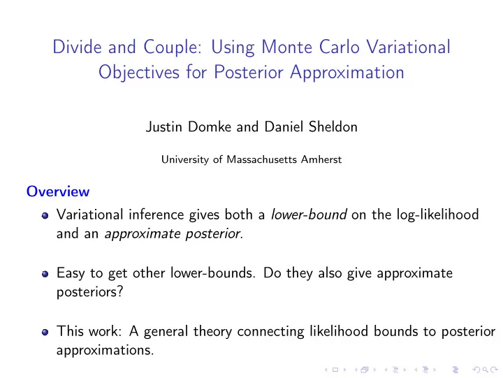
Divide and Couple: Using Monte Carlo Variational Objectives for Posterior Approximation Justin Domke and Daniel Sheldon University of Massachusetts Amherst Overview Variational inference gives both a lower-bound on the log-likelihood and an approximate posterior . Easy to get other lower-bounds. Do they also give approximate posteriors? This work: A general theory connecting likelihood bounds to posterior approximations.

p ( z , x ) − → z Take p ( z , x ) with x fixed.

p ( z , x ) − → z Take p ( z , x ) with x fixed. Observation : If E R = p ( x ) , then E log R ≤ log p ( x ) .

p ( z , x ) − → z Take p ( z , x ) with x fixed. Observation : If E R = p ( x ) , then E log R ≤ log p ( x ) . Example : Take R = p ( x , z ) q ( z ) for z ∼ q Gaussian, optimize q .

log R = 0.237 p ( z , x ) q ( z ) , naive − → z Take p ( z , x ) with x fixed. Observation : If E R = p ( x ) , then E log R ≤ log p ( x ) . Example : Take R = p ( x , z ) q ( z ) for z ∼ q Gaussian, optimize q .

log R = 0.237 p ( z , x ) q ( z ) , naive − → z Take p ( z , x ) with x fixed. Observation : If E R = p ( x ) , then E log R ≤ log p ( x ) . Example : Take R = p ( x , z ) q ( z ) for z ∼ q Gaussian, optimize q . Decomposition : KL ( q ( z ) � p ( z | x )) = log p ( x ) − E log R . Likelihood bound: � Posterior approximation: �

p ( z , x ) Recent work : Better Monte Carlo estimators R .

log R ′ = 0.060 p ( z , x ) q ( z ) , antithetic Recent work : Better Monte Carlo estimators R . Antithetic Sampling : Let T ( z ) “flip” z around mean of q . � p ( z , x )+ p ( T ( z ) , x ) � R = 1 2 q ( z )

log R ′ = 0.060 p ( z , x ) q ( z ) , antithetic Recent work : Better Monte Carlo estimators R . Antithetic Sampling : Let T ( z ) “flip” z around mean of q . � p ( z , x )+ p ( T ( z ) , x ) � R = 1 2 q ( z ) Likelihood bound: � Posterior approximation: × × ×

log R ′ = 0.060 p ( z , x ) q ( z ) , antithetic Recent work : Better Monte Carlo estimators R . Antithetic Sampling : Let T ( z ) “flip” z around mean of q . � p ( z , x )+ p ( T ( z ) , x ) � R = 1 2 q ( z ) Likelihood bound: � Posterior approximation: × × × This paper : Is some other distribution close to p ?

log R ′ = 0.060 p ( z , x ) q ( z ) , antithetic log R ′ = 0.060 p ( z , x ) Q ( z ) , antithetic Contribution of this paper : Given estimator with E R = p ( x ) , we show how to construct Q ( z ) such that KL ( Q ( z ) � p ( z | x )) ≤ log p ( x ) − E log R .

Contribution of this paper : Given estimator with E R = p ( x ) , we show how to construct Q ( z ) such that KL ( Q ( z ) � p ( z | x )) ≤ log p ( x ) − E log R . log R ′ = 0.060 p ( z , x ) q ( z ) , antithetic log R ′ = 0.060 p ( z , x ) Q ( z ) , antithetic

Contribution of this paper : Given estimator with E R = p ( x ) , we show how to construct Q ( z ) such that KL ( Q ( z ) � p ( z | x )) ≤ log p ( x ) − E log R . log R ′ = 0.063 p ( z , x ) q ( z ) , stratified log R ′ = 0.063 p ( z , x ) Q ( z ) , stratified

Contribution of this paper : Given estimator with E R = p ( x ) , we show how to construct Q ( z ) such that KL ( Q ( z ) � p ( z | x )) ≤ log p ( x ) − E log R . log R ′ = 0.021 p ( z , x ) q ( z ) , antithetic within strata log R ′ = 0.021 p ( z , x ) Q ( z ) , antithetic within strata

Contribution of this paper : Given estimator with E R = p ( x ) , we show how to construct Q ( z ) such that KL ( Q ( z ) � p ( z | x )) ≤ log p ( x ) − E log R . How?

Contribution of this paper : Given estimator with E R = p ( x ) , we show how to construct Q ( z ) such that KL ( Q ( z ) � p ( z | x )) ≤ log p ( x ) − E log R . Unbiased estimator: Where is z ? ω R ( ω ) = p ( x ) E

Contribution of this paper : Given estimator with E R = p ( x ) , we show how to construct Q ( z ) such that KL ( Q ( z ) � p ( z | x )) ≤ log p ( x ) − E log R . Unbiased estimator: Where is z ? ω R ( ω ) = p ( x ) E We suggest: Need a coupling : ω R ( ω ) a ( z | ω ω ) = p ( z , x ) E ω � �� � coupling

Contribution of this paper : Given estimator with E R = p ( x ) , we show how to construct Q ( z ) such that KL ( Q ( z ) � p ( z | x )) ≤ log p ( x ) − E log R . Unbiased estimator: Where is z ? ω R ( ω ) = p ( x ) E We suggest: Need a coupling : ω R ( ω ) a ( z | ω ω ) = p ( z , x ) E ω � �� � coupling Then, exist augmented distributions s.t. KL ( Q ( z , ω ω ) � p ( z , ω ω | x )) = log p ( x ) − E log R ω ω

Contribution of this paper : Given estimator with E R = p ( x ) , we show how to construct Q ( z ) such that KL ( Q ( z ) � p ( z | x )) ≤ log p ( x ) − E log R . Summary : Tightening a bound log p ( x ) − E log R is equivalent to VI in an augmented state space ( ω ω , z ) . ω To sample from Q ( z ) draw ω then z ∼ a ( z | ω ) . Paper gives couplings for: ◮ Antithetic sampling ◮ Stratified sampling ◮ Quasi Monte Carlo ◮ Latin hypercube sampling ◮ Arbitrary recursive combinations of above

Implementation : Different sampling methods with Gaussian q .

Experiments confirm : Better likelihood bounds ⇔ better posteriors Poster : Tue Dec 10th, 5:30-7:30pm @ East Exhibition Hall B + C #166