? Quantum Variational Monte Carlo Problem statement Minimize the - PowerPoint PPT Presentation

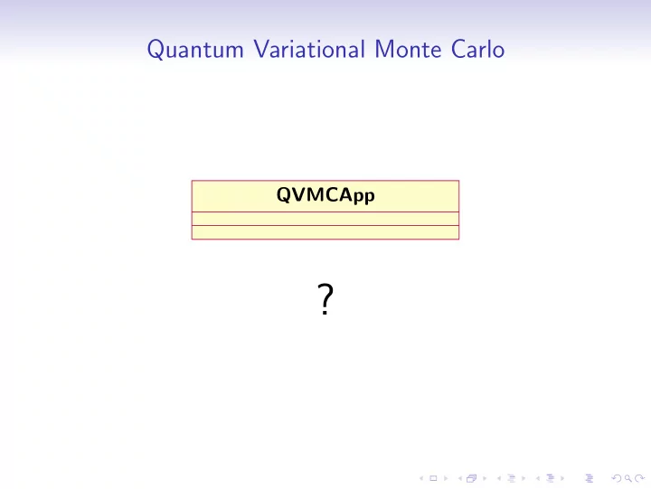
Quantum Variational Monte Carlo QVMCApp ?

Quantum Variational Monte Carlo Problem statement • Minimize the functional E [Ψ T ], where T ( R ) ˆ � d R Ψ ∗ H Ψ T ( R ) E [Ψ T ] = . (1) � d R | Ψ T ( R ) | 2 • The variational principle gives us a lower bound on the ground state energy. E 0 ≤ E [Ψ T ] Need to calculate the integral in (1) .

Quantum Variational Monte Carlo Problem statement • Minimize the functional E [Ψ T ], where T ( R ) ˆ � d R Ψ ∗ H Ψ T ( R ) E [Ψ T ] = . (1) � d R | Ψ T ( R ) | 2 • The variational principle gives us a lower bound on the ground state energy. E 0 ≤ E [Ψ T ] Need to calculate the integral in (1) .

Quantum Variational Monte Carlo Integration QVMCApp Integration ?

Quantum Variational Monte Carlo Monte Carlo integration • Rewrite the integral using the local energy E L and its pdf ρ ( R ) � E [Ψ T ] = d R E L ( R ) ρ ( R ) where ˆ | Ψ T ( R ) | 2 H Ψ T ( R ) E L ( R ) = Ψ T ( R ) , ρ ( R ) = d R ′ | Ψ T ( R ′ ) | 2 . (2) � Sample the local energy following ρ ( R ) .

Quantum Variational Monte Carlo Monte Carlo integration • Rewrite the integral using the local energy E L and its pdf ρ ( R ) � E [Ψ T ] = d R E L ( R ) ρ ( R ) where ˆ | Ψ T ( R ) | 2 H Ψ T ( R ) E L ( R ) = Ψ T ( R ) , ρ ( R ) = d R ′ | Ψ T ( R ′ ) | 2 . (2) � Sample the local energy following ρ ( R ) .

Quantum Variational Monte Carlo Random walkers Metropolis algorithm Metropolis Hastings algorithm for i = 0 , . . . , ncycles for i = 0 , . . . , ncycles for j = 1 , . . . , N for j = 1 , . . . , N F ← 2 ∇ Ψ T ( R ) X ∈ [ − l , l ] Ψ T ( R ) R ′ ← R + X X ∈ gaussian () √ R ′ = R + D ∆ tF + X ∆ t p ← | Ψ T ( R ′ ) | 2 p ← | Ψ T ( R ′ ) | 2 | Ψ T ( R ) | 2 | Ψ T ( R ) | 2 if Y ≤ p , Y ∈ [0 , 1] ω RR ′ = exp ( − ( R ′ − R − D ∆ tF ) 2 ) R = R ′ 4 D ∆ t q ← ω R ′ R ω RR ′ p end if if Y ≤ q , Y ∈ [0 , 1] end for R = R ′ Update statistics end if end for end for Update statistics end for Need wavefunction, quantum force and local energy

Quantum Variational Monte Carlo Random walkers Metropolis algorithm Metropolis Hastings algorithm for i = 0 , . . . , ncycles for i = 0 , . . . , ncycles for j = 1 , . . . , N for j = 1 , . . . , N F ← 2 ∇ Ψ T ( R ) X ∈ [ − l , l ] Ψ T ( R ) R ′ ← R + X X ∈ gaussian () √ R ′ = R + D ∆ tF + X ∆ t p ← | Ψ T ( R ′ ) | 2 p ← | Ψ T ( R ′ ) | 2 | Ψ T ( R ) | 2 | Ψ T ( R ) | 2 if Y ≤ p , Y ∈ [0 , 1] ω RR ′ = exp ( − ( R ′ − R − D ∆ tF ) 2 ) R = R ′ 4 D ∆ t q ← ω R ′ R ω RR ′ p end if if Y ≤ q , Y ∈ [0 , 1] end for R = R ′ Update statistics end if end for end for Update statistics end for Need wavefunction, quantum force and local energy

Quantum Variational Monte Carlo Ingredients for integration QVMCApp QuantumForce Integration Hamiltonian Wavefunction

Quantum Variational Monte Carlo Sample the local energy • The local energy depends on the Hamiltonian. N −∇ 2 � ˆ i + ˆ V + ˆ H = H int , (3) 2 i =1 giving N −∇ 2 ˆ ˆ i Ψ T ( R ) V Ψ T ( R ) H int Ψ T ( R ) � E L ( R ) = + Ψ T ( R ) + . (4) 2Ψ T ( R ) Ψ T ( R ) i =1 Need wavefunction with value and laplacian, in additon to a potential and an interaction.

Quantum Variational Monte Carlo Sample the local energy • The local energy depends on the Hamiltonian. N −∇ 2 � ˆ i + ˆ V + ˆ H = H int , (3) 2 i =1 giving N −∇ 2 ˆ ˆ i Ψ T ( R ) V Ψ T ( R ) H int Ψ T ( R ) � E L ( R ) = + Ψ T ( R ) + . (4) 2Ψ T ( R ) Ψ T ( R ) i =1 Need wavefunction with value and laplacian, in additon to a potential and an interaction.

Quantum Variational Monte Carlo Complete framework QVMCApp Integration Hamiltonian QForce Potential Interaction Wavefunction Kinetic value(r : coordinate) ratio(r new, r old : coordinate) gradient(r : coordinate) laplacian(r : coordinate)

Class definition Integration UML diagram Type declaration Integration 1 TYPE, PUBLIC :: metropolis 2 TYPE (coordinate) :: old, new Metropolis 3 CLASS (hamiltonian), POINTER :: energy => NULL() 4 CLASS (wavefunction), POINTER :: trial_wf => NULL() old, new : coordinate 5 CONTAINS energy : hamiltonian 6 PROCEDURE :: init => metropolis_init trial wf : wavefunction 7 PROCEDURE :: run => metropolis_run init() 8 PROCEDURE :: teardown => metropolis_teardown run() 9 PROCEDURE, PRIVATE :: update_statistics teardown() 10 END TYPE metropolis update statistics() 11 TYPE(metropolis) :: a1 12 13 TYPE, PUBLIC, EXTENDS(metropolis) :: metropolis_hastings 14 CLASS (quantum_force), POINTER :: quantum_force => NULL( MetropolisHastings 15 CONTAINS 16 PROCEDURE :: init => metropolis_hastings_init quantum force : quantum force 17 PROCEDURE :: run => metropolis_hastings_run init() 18 PROCEDURE :: teardown => metropolis_hastings_teardown run() 19 END TYPE metropolis_hastings teardown() 20 TYPE(metropolis_hastings) :: a3

Two dimensional quantum dot Problem statement • Hamiltonian N N � − 1 i + 1 � 1 � 2 ∇ 2 2 ω 2 r 2 � ˆ H = + , (5) i r ij i =1 i < j =1 • Trial wavefunction Ψ T = Ψ D Ψ J , (6) where � � ϕ 1 ( r 1 ) . . . ϕ 1 ( r N ) � � 1 � . . � ... . . Ψ D = √ (7) � � . . � � N ! � � ϕ N ( r 1 ) . . . ϕ N ( r N ) � � and � a ij r ij N � � Ψ J = exp . (8) 1 + β r ij i < j =1

Two dimensional quantum dot Problem statement • Spin independent Hamiltonian means we can split the Slater determinant in a spin up part and a spin down part Ψ D ≈ Ψ ↑ · Ψ ↓ , (9) where � � ϕ 2 ( r 2 ) ϕ 2 ( r 4 ) . . . ϕ 2 ( r N ) � � � � ϕ 4 ( r 2 ) ϕ 4 ( r 4 ) . . . ϕ 4 ( r N ) 1 � � Ψ ↑ = (10) � . . � ... . . � � � ( N / 2)! . . � � � � ϕ N ( r 2 ) ϕ N ( r 4 ) . . . ϕ N ( r N ) � � and � � ϕ 1 ( r 1 ) ϕ 1 ( r 3 ) . . . ϕ 1 ( r N − 1 ) � � � � ϕ 3 ( r 1 ) ϕ 3 ( r 3 ) . . . ϕ 3 ( r N − 1 ) 1 � � Ψ ↓ = . (11) � . . � ... . . � � � ( N / 2)! . . � � � � ϕ N − 1 ( r 1 ) ϕ N − 1 ( r 3 ) . . . ϕ N − 1 ( r N − 1 ) � �

Two dimensional quantum dot Complete wavefunction framework Wavefunction ExpFactor Determinant Jastrow SpState Hermite

Class definition Wavefunction UML diagram Type declaration Wavefunction TYPE, PUBLIC, EXTENDS(wavefunction) :: variational CLASS (exponential_wavefunction), POINTER :: exp_factor variational CLASS (jastrow), POINTER :: jastrow_factor => NULL() exp factor : exponential wavefunction CONTAINS jastrow factor : jastrow PROCEDURE get => variational_get PROCEDURE gradient => variational_gradient get() PROCEDURE laplacian => variational_laplacian gradient() END TYPE variational laplacian() ratio() TYPE, PUBLIC, EXTENDS(variational) :: determinental CLASS (determinant_none), POINTER :: determinant => NULL CONTAINS PROCEDURE get => determinental_get determinental PROCEDURE gradient => determinental_gradient determinant : determinant none PROCEDURE laplacian => determinental_laplacian PROCEDURE ratio => determinental_ratio get() END TYPE determinental gradient() laplacian() ratio()

Profiling with grof • Compile your code with the -pg option. • Run your code. • Run gprof: gprof ./exeutable ¿ outputfile • Study outputfile