Divide-and-Conquer Lecturer: Shi Li Department of Computer Science - PowerPoint PPT Presentation
CSE 431/531: Analysis of Algorithms Divide-and-Conquer Lecturer: Shi Li Department of Computer Science and Engineering University at Buffalo Outline Divide-and-Conquer 1 Counting Inversions 2 Quicksort and Selection 3 Quicksort Lower
CSE 431/531: Analysis of Algorithms Divide-and-Conquer Lecturer: Shi Li Department of Computer Science and Engineering University at Buffalo
Outline Divide-and-Conquer 1 Counting Inversions 2 Quicksort and Selection 3 Quicksort Lower Bound for Comparison-Based Sorting Algorithms Selection Problem Polynomial Multiplication 4 Other Classic Algorithms using Divide-and-Conquer 5 Solving Recurrences 6 Self-Balancing Binary Search Trees 7 Computing n -th Fibonacci Number 8 2/95
Greedy algorithm: design efficient algorithms Divide-and-conquer: design more efficient algorithms 3/95
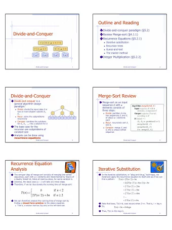
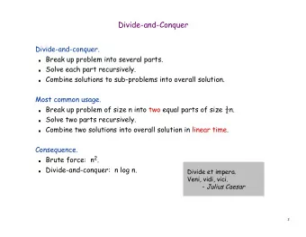
Divide-and-Conquer Divide : Divide instance into many smaller instances Conquer : Solve each of smaller instances recursively and separately Combine : Combine solutions to small instances to obtain a solution for the original big instance 4/95
merge-sort ( A, n ) if n = 1 then 1 return A 2 else 3 � � � � B ← merge-sort A 1 .. ⌊ n/ 2 ⌋ , ⌊ n/ 2 ⌋ 4 � � � � C ← merge-sort A ⌊ n/ 2 ⌋ + 1 ..n , ⌈ n/ 2 ⌉ 5 return merge ( B, C, ⌊ n/ 2 ⌋ , ⌈ n/ 2 ⌉ ) 6 Divide: trivial Conquer: 4 , 5 Combine: 6 5/95
Running Time for Merge-Sort A [1 .. 8] A [1 .. 4] A [5 .. 8] A [1 .. 2] A [3 .. 4] A [5 .. 6] A [7 .. 8] A [1] A [2] A [3] A [4] A [5] A [6] A [7] A [8] Each level takes running time O ( n ) There are O (lg n ) levels Running time = O ( n lg n ) Better than insertion sort 6/95
Running Time for Merge-Sort Using Recurrence T ( n ) = running time for sorting n numbers,then � O (1) if n = 1 T ( n ) = T ( ⌊ n/ 2 ⌋ ) + T ( ⌈ n/ 2 ⌉ ) + O ( n ) if n ≥ 2 With some tolerance of informality: � O (1) if n = 1 T ( n ) = 2 T ( n/ 2) + O ( n ) if n ≥ 2 Even simpler: T ( n ) = 2 T ( n/ 2) + O ( n ) . (Implicit assumption: T ( n ) = O (1) if n is at most some constant.) Solving this recurrence, we have T ( n ) = O ( n lg n ) (we shall show how later) 7/95
Outline Divide-and-Conquer 1 Counting Inversions 2 Quicksort and Selection 3 Quicksort Lower Bound for Comparison-Based Sorting Algorithms Selection Problem Polynomial Multiplication 4 Other Classic Algorithms using Divide-and-Conquer 5 Solving Recurrences 6 Self-Balancing Binary Search Trees 7 Computing n -th Fibonacci Number 8 8/95
Def. Given an array A of n integers, an inversion in A is a pair ( i, j ) of indices such that i < j and A [ i ] > A [ j ] . Counting Inversions Input: an sequence A of n numbers Output: number of inversions in A Example: 10 8 15 9 12 8 9 10 12 15 4 inversions (for convenience, using numbers, not indices): (10 , 8) , (10 , 9) , (15 , 9) , (15 , 12) 9/95
Naive Algorithm for Counting Inversions count-inversions ( A, n ) c ← 0 1 for every i ← 1 to n − 1 2 for every j ← i + 1 to n 3 if A [ i ] > A [ j ] then c ← c + 1 4 return c 5 10/95
Divide-and-Conquer p A : B C p = ⌊ n/ 2 ⌋ , B = A [1 ..p ] , C = A [ p + 1 ..n ] # invs ( A ) = # invs ( B ) + # invs ( C ) + m � �� �� m = ( i, j ) : B [ i ] > C [ j ] � Q: How fast can we compute m , via trivial algorithm? A: O ( n 2 ) Can not improve the O ( n 2 ) time for counting inversions. 11/95
Divide-and-Conquer p A : B C p = ⌊ n/ 2 ⌋ , B = A [1 ..p ] , C = A [ p + 1 ..n ] # invs ( A ) = # invs ( B ) + # invs ( C ) + m � �� �� m = ( i, j ) : B [ i ] > C [ j ] � Lemma If both B and C are sorted, then we can compute m in O ( n ) time! 12/95
Counting Inversions between B and C Count pairs i, j such that B [ i ] > C [ j ] : B : total= 0 18 2 2 8 5 13 3 8 12 20 32 48 C : 5 7 9 25 29 +0 +2 +3 +3 +5 +5 3 8 12 20 32 48 5 7 9 25 29 13/95
Count Inversions between B and C Procedure that merges B and C and counts inversions between B and C at the same time merge-and-count ( B, C, n 1 , n 2 ) count ← 0 ; 1 A ← [] ; i ← 1 ; j ← 1 2 while i ≤ n 1 or j ≤ n 2 3 if j > n 2 or ( i ≤ n 1 and B [ i ] ≤ C [ j ] ) then 4 append B [ i ] to A ; i ← i + 1 5 count ← count + ( j − 1) 6 else 7 append C [ j ] to A ; j ← j + 1 8 return ( A, count ) 9 14/95
Sort and Count Inversions in A A procedure that returns the sorted array of A and counts the number of inversions in A : sort-and-count( A, n ) Divide: trivial if n = 1 then Conquer: 4 , 5 1 return ( A, 0) Combine: 6 , 7 2 else 3 � � � � ( B, m 1 ) ← sort-and-count A 1 .. ⌊ n/ 2 ⌋ , ⌊ n/ 2 ⌋ 4 � � � � ( C, m 2 ) ← sort-and-count A ⌊ n/ 2 ⌋ + 1 ..n , ⌈ n/ 2 ⌉ 5 ( A, m 3 ) ← merge-and-count ( B, C, ⌊ n/ 2 ⌋ , ⌈ n/ 2 ⌉ ) 6 return ( A, m 1 + m 2 + m 3 ) 7 15/95
sort-and-count( A, n ) if n = 1 then 1 return ( A, 0) 2 else 3 � � � � ( B, m 1 ) ← sort-and-count A 1 .. ⌊ n/ 2 ⌋ , ⌊ n/ 2 ⌋ 4 � � � � ( C, m 2 ) ← sort-and-count A ⌊ n/ 2 ⌋ + 1 ..n , ⌈ n/ 2 ⌉ 5 ( A, m 3 ) ← merge-and-count ( B, C, ⌊ n/ 2 ⌋ , ⌈ n/ 2 ⌉ ) 6 return ( A, m 1 + m 2 + m 3 ) 7 Recurrence for the running time: T ( n ) = 2 T ( n/ 2) + O ( n ) Running time = O ( n lg n ) 16/95
Outline Divide-and-Conquer 1 Counting Inversions 2 Quicksort and Selection 3 Quicksort Lower Bound for Comparison-Based Sorting Algorithms Selection Problem Polynomial Multiplication 4 Other Classic Algorithms using Divide-and-Conquer 5 Solving Recurrences 6 Self-Balancing Binary Search Trees 7 Computing n -th Fibonacci Number 8 17/95
Outline Divide-and-Conquer 1 Counting Inversions 2 Quicksort and Selection 3 Quicksort Lower Bound for Comparison-Based Sorting Algorithms Selection Problem Polynomial Multiplication 4 Other Classic Algorithms using Divide-and-Conquer 5 Solving Recurrences 6 Self-Balancing Binary Search Trees 7 Computing n -th Fibonacci Number 8 18/95
Quicksort vs Merge-Sort Merge Sort Quicksort Divide Trivial Separate small and big numbers Conquer Recurse Recurse Combine Merge 2 sorted arrays Trivial 19/95
Quicksort Example Assumption We can choose median of an array of size n in O ( n ) time. 29 82 75 64 64 38 45 94 69 25 76 15 92 37 17 85 29 29 38 45 25 15 37 17 64 82 75 94 92 69 76 85 25 15 17 29 38 45 37 64 82 75 94 92 69 76 85 20/95
Quicksort quicksort ( A, n ) if n ≤ 1 then return A 1 x ← lower median of A 2 A L ← elements in A that are less than x \\ Divide 3 A R ← elements in A that are greater than x \\ Divide 4 B L ← quicksort ( A L , A L . size ) \\ Conquer 5 B R ← quicksort ( A R , A R . size ) \\ Conquer 6 t ← number of times x appear A 7 return the array obtained by concatenating B L , the array 8 containing t copies of x , and B R Recurrence T ( n ) ≤ 2 T ( n/ 2) + O ( n ) Running time = O ( n lg n ) 21/95
Assumption We can choose median of an array of size n in O ( n ) time. Q: How to remove this assumption? A: There is an algorithm to find median in O ( n ) time, using 1 divide-and-conquer (we shall not talk about it; it is complicated and not practical) Choose a pivot randomly and pretend it is the median (it is 2 practical) 22/95
Quicksort Using A Random Pivot quicksort ( A, n ) if n ≤ 1 then return A 1 x ← a random element of A ( x is called a pivot) 2 A L ← elements in A that are less than x \\ Divide 3 A R ← elements in A that are greater than x \\ Divide 4 B L ← quicksort ( A L , A L . size ) \\ Conquer 5 B R ← quicksort ( A R , A R . size ) \\ Conquer 6 t ← number of times x appear A 7 return the array obtained by concatenating B L , the array 8 containing t copies of x , and B R 23/95
Randomized Algorithm Model Assumption There is a procedure to produce a random real number in [0 , 1] . Q: Can computers really produce random numbers? A: No! The execution of a computer programs is deterministic! In practice: use pseudo-random-generator, a deterministic algorithm returning numbers that “look like” random In theory: make the assumption 24/95
Quicksort Using A Random Pivot quicksort ( A, n ) if n ≤ 1 then return A 1 x ← a random element of A ( x is called a pivot) 2 A L ← elements in A that are less than x \\ Divide 3 A R ← elements in A that are greater than x \\ Divide 4 B L ← quicksort ( A L , A L . size ) \\ Conquer 5 B R ← quicksort ( A R , A R . size ) \\ Conquer 6 t ← number of times x appear A 7 return the array obtained by concatenating B L , the array 8 containing t copies of x , and B R When we talk about randomized algorithm in the future, we show that the expected running time of the algorithm is O ( n lg n ) . 25/95
Quicksort Can Be Implemented as an “In-Place” Sorting Algorithm In-Place Sorting Algorithm: an algorithm that only uses “small” extra space. j i 64 17 64 37 82 15 64 75 29 38 45 94 25 64 64 69 25 64 69 76 94 64 15 92 64 75 37 82 64 17 85 To partition the array into two parts, we only need O (1) extra space. 26/95
Quicksort Can Be Implemented as an “In-Place” Sorting Algorithm partition ( A, ℓ, r ) p ← random integer between ℓ and r 1 swap A [ p ] and A [ ℓ ] 2 i ← ℓ, j ← r 3 while i < j do 4 while i < j and A [ i ] ≤ A [ j ] do j ← j − 1 5 swap A [ i ] and A [ j ] 6 while i < j and A [ i ] ≤ A [ j ] do i ← i + 1 7 swap A [ i ] and A [ j ] 8 return i 9 27/95
Recommend
More recommend
Explore More Topics
Stay informed with curated content and fresh updates.
