Distance Sampling Simulations Overview Why simulate? How it - PowerPoint PPT Presentation
Distance Sampling Simulations Overview Why simulate? How it works Automated survey design Coverage probability Which design? Design trade-offs Defining the population Population description Detectability
Distance Sampling Simulations
Overview Why simulate? How it works Automated survey design Coverage probability Which design? Design trade-offs Defining the population Population description Detectability Example Simulations
Why Simulate? Surveys expensive, simulations cheap! Test different survey designs Test survey protocols Investigate analysis properties Investigate violation of assumptions
How it works Blue rectangles indicate information supplied by the user. Green rectangles are objects created by DSsim in the simulation process. Orange diamonds indicate the processes carried out by DSsim.
How it works Assess: • Bias • Precision • CI coverage Across different designs/ scenarios
Automated Survey Design Generate random sets of transects according to an algorithm Assess design properties Generate multiple transect sets for simulations
Automated Survey Design Coverage Probability P – Uniform coverage probability, π = 1/3 Survey Region P – Uniform coverage probability, π = 1/3 – Uneven coverage for any given realisation
Which Design? Uniformity of coverage probability Even-ness of coverage within any given realisation Overlap of samplers Cost of travel between samplers Efficiency when density varies within the region
Design Trade-Offs Convex hull Survey Region Survey Region Minimum bounding rectangle
Population Definition True population size? Occur as individuals or clusters? Covariates which will affect detectability? How is the population distributed within the study region? Ideally have a previously fitted density surface Otherwise test over a range of plausible distributions
Detectability Distance needs: shape and scale parameters on the natural scale covariate parameters on the log scale
Detectability Golftees project exp(0.268179) = 1.307581 (MCDS) (MRDS) Natural scale Log scale
Detectability In simulation: exp(log(2.622)-0.696) = 1.307265 exp(log(1.307581)+0.696) = 2.622633
Detectability
Analysis Data Filter must specify a right truncation distance Model Definition must be either MRDS or MA MRDS – for fitting a specific model MA – for model selection (Note: MA model definitions require the creation of analyses)
Any questions so far…
Example Simulations To bin or not to bin? Testing pooling robustness in relation to truncation distance. Comparison of subjective and random designs.
To Bin or Not to Bin? Simulation: Generated 999 datasets Added multiplicative measurement error Distance = True Distance * R R = (U + 0.5), where U~Beta( θ , θ ) 1 No error, ~15% CV ( θ = 5), ~30% CV ( θ = 1) Analysed them in difference ways Exact distances, 5 Equal bins, 5 Unequal bins, 3 Equal bins Average number of observations ~ 150 Model selection on minimum AIC Half-normal v Hazard rate 1 Marques T. (2004) Predicting and correcting bias caused by measurement error in line transect sampling using multiplicative error models Biometrics 60:757--763
To Bin or Not to Bin Results Exact 5 Equal Bins 5 Unequal Bins 3 Equal Bins Distances -1.16% bias -1.11% bias -0.16% bias -0.19% bias No Error 210 SE 217 SE 221 SE 255 SE 0.48% bias o.5% bias 1.36% bias 1.72%bias 15% CV 214 SE 221 SE 221 SE 264 SE 6.66% bias 6.61% bias 7.43% bias 8.20% bias 30% CV 237 SE 250 SE 262 SE 338 SE
Pooling Robustness and Truncation DSsim vignette Rectangular study region Systematic parallel transects with a spacing of 1000m
Pooling Robustness and Truncation DSsim vignette Uniform density surface Population size of 200 50% male, 50% female
Pooling Robustness and Truncation DSsim vignette Half-normal shape for detectability Scale parameter of 120 for the females Scale parameter of ~540 for the males
Pooling Robustness and Truncation DSsim vignette Half-normal shape for detectability Scale parameter of 120 for the females Scale parameter of ~540 for the males exp(log(120)+1.5) = 537.8
Pooling Robustness and Truncation DSsim vignette Two types of analyses: hn v hr hn ~ sex Selection criteria: AIC Histogram of data from covariate simulation with manually selected candidate truncation distances.
Pooling Robustness and Truncation Results HN v HR:
Example Simulation
Subjective survey design 337 km effort
Random Designs Mean cyclic track 845 km Mean cyclic track 843 km Mean effort 474 km Mean effort 695 km
Coverage probability Systematic Parallel Design Equal Spaced Zigzag Design
Simulation Generates a realisation of the population based on a fixed N of 1500 Generates a realisation of the design Different each time for the random designs The same each time for the subjective design Simulates the detection process Analyses the results Half-normal Hazard-rate Repeats a number of times
Practical Now attempt the DSsim practical: R version – subjective design and parallel v zig zag Distance version – parallel v zig zag only You will need the library shapefiles.
Recommend
More recommend
Explore More Topics
Stay informed with curated content and fresh updates.
