Discrete Events Simulation Michel Bierlaire - PowerPoint PPT Presentation
Discrete Events Simulation Michel Bierlaire michel.bierlaire@epfl.ch Transport and Mobility Laboratory Discrete Events Simulation p. 1/18 Simulation of a system Generate the stochastic mechanisms of the systems. Collect the
Discrete Events Simulation Michel Bierlaire michel.bierlaire@epfl.ch Transport and Mobility Laboratory Discrete Events Simulation – p. 1/18
Simulation of a system • Generate the stochastic mechanisms of the systems. • Collect the evolution of given indicators over time. • Book-keeping may be complex. • Need for a general framework. Discrete event simulation Discrete Events Simulation – p. 2/18
Discrete Event Simulation Keep track of variables: • Time variable t : amount of time that has elapsed. • Counter variables: count events having occurred by t • System state variables. Events: • List of future events sorted in chronological order • Process the next event: • remove the first event in the list, • update the variables, • generate new events, if applicable (keep the list sorted), • collect statistics. Discrete Events Simulation – p. 3/18
Discrete Event Simulation: an example Example: Satellite • Today, Bilal works alone at the bar at Satellite. • When a customer arrives, she is served if Bilal is free. Otherwise, she joins the queue. • Customers are served using a “first come, first served” logic. • When Bilal has finished serving a customer, • he starts serving the next customer in line, or • waits for the next customer to arrive if the queue is empty. • The amount of time required by Bilal to serve a customer is a random variable X s with pdf f s . • The amount of time between the arrival of two customers is a random variable X a with pdf f a . • Satellite does not accept the arrival of customers after time T . Discrete Events Simulation – p. 4/18
Discrete Event Simulation: an example Possible questions: • In average, how much time does a customer wait after her arrival, until being served? • When can Bilal go home? Discrete Events Simulation – p. 5/18
Discrete Event Simulation: an example Variables: Time: t Counters: number of arrivals N A number of departures N D System state: number of customers in the system n Event list: • Next arrival. Time: t A • Service completion for the customer currently being served. Time: t D ( ∞ if no customer is being served). • The bar closes. Time: T . List management: • The number of events is always 3 in this example. • We just need to update the times, and keep them sorted. Discrete Events Simulation – p. 6/18
Initialization • Time: t = 0 . • Counters: N A = N D = 0 . • State: n = 0 . • First event: arrival of first customer: draw r from f a . • Events list: • t A = r , • t D = ∞ , • T (bar closes). Statistics to collect: • A ( i ) arrival of customer i . • D ( i ) departure of customer i . • T p time after T that the last customer departs. Discrete Events Simulation – p. 7/18
Case 1: arrival of a customer If t A = min( t A , t D , T ) • Time t = t A : we move along to time t A . • Counter N A = N A + 1 : one more customer arrived. • State n = n + 1 : one more customer in the system. • Next arrival: • draw r from f a , • t A = t + r . • Service time: if n = 1 (she is served immediately) • draw s from f s , • t D = t + s . • Statistics: A ( N A ) = t . Discrete Events Simulation – p. 8/18
Case 2: departure of a customer Conditions: t D = min( t A , t D , T ) , t D < t A • Time t = t D : we move along to time t D . • Counter N D = N D + 1 : one more customer departed. • State n = n − 1 : one less customer in the system. • Service time: if n = 0 , then t D = ∞ . Otherwise, • draw s from f s , • t D = t + s . • Statistics: D ( N D ) = t . Discrete Events Simulation – p. 9/18
Case 3: after hours Conditions: T < min( t A , t D ) , 1. Customers are still waiting: n > 0 • Time t = t D : we move along to time t D . • Counter N D = N D + 1 : one more customer departed. • State n = n − 1 : one less customer in the system. • Service time: if n > 0 , then • draw s from f s , • t D = t + s . • Statistics: D ( N D ) = t . 2. No more customers: n = 0 • Statistics: T p = max( t − T, 0) . Discrete Events Simulation – p. 10/18
An instance Scenario: • Service time: exponential with mean 1.0 • Inter-arrival time: exponential with mean 1.0 • Closing time: 10.0 Discrete Events Simulation – p. 11/18
An instance (ctd.) Event t NA ND n tA tD T Arrival 0.94 1 0 1 1.48 3.22 10.0 Arrival 1.48 2 0 2 2.01 3.22 10.0 Arrival 2.01 3 0 3 3.16 3.22 10.0 Arrival 3.16 4 0 4 3.44 3.22 10.0 Departure 3.22 4 1 3 3.44 3.49 10.0 Arrival 3.44 5 1 4 3.81 3.49 10.0 Departure 3.49 5 2 3 3.81 3.91 10.0 Arrival 3.81 6 2 4 7.22 3.91 10.0 Departure 3.91 6 3 3 7.22 5.84 10.0 Departure 5.84 6 4 2 7.22 5.88 10.0 Departure 5.88 6 5 1 7.22 6.49 10.0 Departure 6.49 6 6 0 7.22 10.0 ∞ Arrival 7.22 7 6 1 7.42 7.38 10.0 . . . Discrete Events Simulation – p. 12/18
An instance (ctd.) Event t NA ND n tA tD T . . . Departure 7.38 7 7 0 7.42 10.0 ∞ Arrival 7.42 8 7 1 8.58 8.42 10.0 Departure 8.42 8 8 0 8.58 10.0 ∞ Arrival 8.58 9 8 1 9.64 9.91 10.0 Arrival 9.64 10 8 2 10.7 9.91 10.0 Departure 9.91 10 9 1 10.7 10.7 10.0 After hours 10.7 10 10 0 10.7 10.7 10.0 Finish 10.7 10 10 0 10.7 10.7 10.0 Discrete Events Simulation – p. 13/18
An instance (ctd.) Statistics for each customer (rounded): Cust. Arrival Departure Time 1 0.94 3.22 2.28 2 1.48 3.49 2.02 3 2.01 3.91 1.9 4 3.16 5.84 2.68 5 3.44 5.88 2.45 6 3.81 6.49 2.68 7 7.22 7.38 0.165 8 7.42 8.42 1.0 9 8.58 9.91 1.33 10 9.64 10.7 1.02 • Average time in the system: 1.75 • Bilal leaves Satellite at 10.7 Discrete Events Simulation – p. 14/18
Another instance Scenario: Bilal works faster • Service time: exponential with mean 0.2 • Inter-arrival time: exponential with mean 1.0 • Closing time: 10.0 Discrete Events Simulation – p. 15/18
An instance (ctd.) Event t NA ND n tA tD T Arrival 1.02 1 0 1 3.14 1.38 10.0 Departure 1.38 1 1 0 3.14 10.0 ∞ Arrival 3.14 2 1 1 6.97 3.25 10.0 Departure 3.25 2 2 0 6.97 10.0 ∞ Arrival 6.97 3 2 1 7.08 7.26 10.0 Arrival 7.08 4 2 2 7.24 7.26 10.0 Arrival 7.24 5 2 3 10.0 7.26 10.0 Departure 7.26 5 3 2 10.0 8.32 10.0 Departure 8.32 5 4 1 10.0 8.51 10.0 Departure 8.51 5 5 0 10.0 10.0 ∞ Finish 10.0 5 5 0 10.0 10.0 ∞ Discrete Events Simulation – p. 16/18
An instance (ctd.) Statistics for each customer (rounded): Cust. Arrival Departure Time 1 1.02 1.38 0.355 2 3.14 3.25 0.11 3 6.97 7.26 0.296 4 7.08 8.32 1.24 5 7.24 8.51 1.27 • Average time in the system: 0.654 • Bilal leaves Satellite at 10.0. • He stops working at 8.51. Discrete Events Simulation – p. 17/18
Notes • The indicators under interest are random variables. • Running the simulator provides one realization of these r.v. • A large number of realizations must be drawn to have an idea of the distribution. • It is not unusual to have indicators with complex distribution, that is multi-modal and asymmetric. Therefore, the mean may not always be sufficient to describe the r.v. Discrete Events Simulation – p. 18/18
Recommend
More recommend
Explore More Topics
Stay informed with curated content and fresh updates.
