Diffusion Approximations for Ecological Models by Phil Pollett - PDF document
Diffusion Approximations for Ecological Models by Phil Pollett The University of Queensland Zen Maxims for Survival in a Modern University Those not relevant to my talk Dont be irreplaceable; if you cant be re- placed, you cant
Diffusion Approximations for Ecological Models by Phil Pollett The University of Queensland
Zen Maxims for Survival in a Modern University Those not relevant to my talk • Don’t be irreplaceable; if you can’t be re- placed, you can’t be promoted. • Give a man a fish and he will eat for a day; teach him how to fish, and he will sit in a boat and drink beer all day. • If you lend someone $20, and never see them again, it was probably worth it. • If you tell the truth, you don’t need a good memory. • A closed mouth gathers no foot. 2
Zen Maxims for Survival in a Modern University Those relevant to my talk • Good judgement comes from bad experi- ence, and a lot of that comes from bad judgement. • It may be that your sole purpose in life is simply to serve as a warning to others. • Before you criticize someone, you should walk a mile in their shoes; that way, when you do criticize them, you’ll be a mile away and you’ll have their shoes. 3
DIFFUSION APPROXIMATIONS Technical definition. A diffusion process is a continuous-time (strong) Markov process whose sample path X ( t ) is an almost-surely continu- ous function of t . Sample path of a diffusion model for population density 0.6 0.55 0.5 0.45 Population density X(t) 0.4 0.35 0.3 0.25 0.2 0.15 0.1 0 10 20 30 40 50 60 70 80 90 100 Time t Diffusion processes are usually realised as ap- proximations of jump processes (in discrete or continuous time) by way of a limiting proce- √ dure involving space-time scaling: ∆ x ∼ ∆ t . 4
Why are they useful models? They are pop- ular in ecological modelling because their pa- rameters can be estimated simply from very little data, and they offer explicit expressions for important quantities of interest, such as the expected time to extinction. Formulae arising from diffusion Difficulties. models are frequently used in situations where this is clearly inappropriate: • The underlying process, which the diffusion is approximating, might not itself be appro- priate for modelling the system in question. • The approximation procedure is often not well understood, and its physical meaning not taken into account. • The diffusion approximation might provide estimates that are at variance with the un- derlying model. 5
EXAMPLE The stochastic logistic model . This model is ubiquitous in the literature on population modelling, but also appears in a variety of dif- ferent contexts: for example, chemical kinet- ics, genetics and epidemics. It is a birth-death process n ( t ) taking values in S = { 0 , 1 , . . . , N } with birth and death rates q ( n, n + 1) = λ N n ( N − n ) q ( n, n − 1) = µn , where N is to be interpretted as the carrying capacity and λ, µ > 0. Absorption at state 0 (representing the event of extinction) occurs with probability 1. We will consider the inter- esting case of positive drift: λ > µ . A diffusion approximation . There is a dif- fusion approximation for the density X ( t ) = n ( t ) /N , which becomes more and more accu- rate as N gets large. 6
Illustration . Here is a simulation of the lo- gistic model, together with its diffusion ap- proximation ( N = 500, λ = 0 . 2, µ = 0 . 1 and X (0) = x 0 = 0 . 1): 0.6 0.55 0.5 0.45 0.4 Population density 0.35 0.3 0.25 0.2 0.15 0.1 0 10 20 30 40 50 60 70 80 90 100 Time The mean path is shown (solid), with ± two standard deviations (dashed). 7
Specification of the approximation . X ( t ) � � µ t , σ 2 has an approximate normal N dist- t /N ribution, where qx 0 µ t = x 0 + ( q − x 0 ) e − λqt , t ≥ 0 , q = 1 − ρ , ρ = µ/λ ( < 1), and � t σ 2 t = M 2 � G ( µ s ) /M 2 � ds , t s 0 where G ( x ) = λx (1 − x ) + µx , 0 ≤ x ≤ 1, and q 2 e − λqt M t = ( x 0 + ( q − x 0 ) e − λqt ) 2 . Note that σ 2 t → ρ and t → ∞ . Note also that q is an equilibrium point, which is asymptotically stable ( µ t → q ). It can be shown that σ 2 t = ρ (1 − e − 2 λqt ) + O ( | x 0 − q | ) , for x 0 near q . 8
Extinction times . The diffusion approxima- tion accurately models the density X ( t ), but how good is it in predicting extinction times? Let τ i be the expected time to extinction start- ing in state i . 500 450 400 350 Expected time to extinction 300 250 200 150 100 50 0 0 0.1 0.2 0.3 0.4 0.5 0.6 0.7 0.8 0.9 1 x The approximation (dashed) for τ i is show, to- gether with the exact values (solid) obtain di- rectly from the logistic model ( N = 100, λ = 0 . 1111, µ = 0 . 1, n (0) = n 0 = i , x 0 = x = i/N ). 9
8 12 x 10 10 8 Expected time to extinction 6 4 2 0 180 185 190 195 200 205 210 215 220 225 230 N Shown is the diffusion approximation (dashed) for τ i , the exact values (solid) and a large- N asymptotic expansion (dash-dot): N � e − (1 − ρ ) τ i ∼ ρ (1 − ρ i ) 2 π N . µ (1 − ρ ) 2 ρ ( ρ = 0 . 1538, µ = 0 . 1, x 0 = 0 . 05, and n 0 = i = [0 . 05 × N ].) 10
PAPER IN THE PROCEEDINGS We identify a class of Markovian models (called asymptotically density dependent models) that permit a diffusion approximation through a sim- ple limiting procedure. This procedure allows one to immediately identify the most appropri- ate approximating diffusion and to decide whe- ther the diffusion approximation is appropriate for describing the population in question. Re- sult are presented in a form that most easily permits their direct application to population models. Additionally, results are presented that allow one to assess the accuracy of diffusion approx- imations by specifying for how long and over what ranges the underlying Markovian model is faithfully approximated. The logistic model is considered in detail. In addition to diffusion approximations, several exact methods are presented, which are use- ful outside this context. 11
Recommend
More recommend
Explore More Topics
Stay informed with curated content and fresh updates.
