Diffusion approximation as a tool in computer networks performance - PowerPoint PPT Presentation

Diffusion approximation as a tool in computer networks performance evaluation CNT 2500 Tadeusz Czachórski tadek@iitis.pl https://www.iitis.pl/en/person/tczachorski Institute of Theoretical and Applied Informatics of Polish Academy of Sciences, Gliwice, Poland The 9th International Conference on Electronics, Communications and Networks CECNet 2019, October 18-21, 2019 Kitakyushu City, Japan

Introduction • Since Erlang and Engset times, queueing models are extensively used to model telephone, computer and telecommunication networks. • The rapid growth of telephone switching systems in offices of public switch telephone networks (PSTN), mobile switching centers (MSC) and radio access networks of cellular mobile networks, cloud data center systems and customer service centers has renewed the interest in multiserver queueing models • Markov chain models consider events thus have limitations (explosion of the number of states), we propose steady state and transient state diffusion approximation models based on changes of flows, giving numerical results. • We concentrate on the G/G/c/c+K queueing model (Kendal’s notation) having in mind design and performance evaluation of multichannel communication networks.

Queueing model, generic problem server "customers" input flow output flow queue Known: − arrival pattern, e.g. interarrival time distribution − service time, e.g. service time distribution − queueing discipline − queue size limitations To determine: − queue distribution (or its moments) − waiting time distribution (or its moments) − losses (if limited queue)

Some Applications of G/G/c/c+K models G/G/c/c+K queueing model Radio access channels 1 2 Transmission queue λ . . . . . . c Figure 1: Queueing model for the LTE radio access downlink

G/G/c/c+K queueing model transmission unit packet aggregation bufffers λ (1) 1 λ (2) λ 1 Burst transmission buffer λ (3) 2 λ 2 . . . . . . . . . . . . λ n c λ ( k ) Figure 2: Queueing model of the edge node in optical burst switching networks

G/G/c/c+K queing model Physical machines PS1 λ 1 Task scheduler Task queue PS2 λ 2 · · · λ N · · · PSc Figure 3: Simplified queuing Model of a Cloud Data Center

Figure 4: Queuing model of the UPnP/HTTP network

Figure 5: Evaluation of an Polish Insurance (ZUS) Database System

Figure 6: Queuing model of the Database System

Diffusion approximation approach to G/G/c/c + K model Diffusion approximation is a method introduced to queueing theory by H. Kobayashi and E. Gelenbe in 1970’s. Our diffusion G/G/c/c+K model is an extension of Gelenbe’s G/G/1/K model presented in [ On approximate computer system models , E. Gelenbe, Journal of the ACM (JACM), 1975]. We adapt it to multiple channel and finite population case where required diffusion parameters are state-dependent. We provide also transient state analysis in case of time dependent flows or the change of working channels to see how the queues and blocking probability vary with time and what is the dynamics of the overflow traffic.

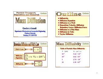
The essence of diffusion approximation is the replacement of a stochastic process N ( t ) – the number of customers in a queueing system by a diffusion process X ( t ) . The diffusion equation ∂ 2 f ( x, t ; x 0 ) ∂f ( x, t ; x 0 ) = α − β ∂f ( x, t ; x 0 ) . ∂x 2 ∂t 2 ∂x with appropriate parameters and boundary conditions determines the probability density function f ( x, t ; x 0 ) of the process and this function is an approximation of the distribution of the number of customers in the service system

The choice of diffusion parameters Let A ( x ) , B ( x ) denote the interarrival and service time distributions. The distributions are general but not specified, the method requires only their two first moments: means E [ A ] = 1 /λ , E [ B ] = 1 /µ and variances Var [ A ] = σ 2 A , Var [ B ] = σ 2 B . Denote also squared coefficients of variation C 2 A = σ 2 A λ 2 , C 2 B = σ 2 B µ 2 . The changes of N ( t ) during ∆ are normally distributed with mean A λ 3 + σ 2 ( λ − µ )∆ , and variance ( σ 2 B µ 3 )∆ = ( C 2 A λ + C 2 B µ )∆ . The changes of X ( t ) in dt are normally distributed with mean βdt and variance αdt .

Therefore in G/G/ 1 /N model the choice of diffusion parameters is [Gelenbe] β = λ − µ, A λ 3 + σ 2 B µ 3 = C 2 α = σ 2 A λ + C 2 B µ These values assure that the processes N ( t ) and X ( t ) have not only normally distributed changes but also their mean and variance increase in the same way with the observation time.

The choice of boundary conditons In case of G/G/ 1 /N queue, the diffusion process should be limited to the interval [0 , N ] corresponding to possible number of customers inside the system. To ensure it, two barriers are placed at x = 0 and x = N . In Gelenbe’s model when the diffusion process comes to x = 0 , it remains there for a time exponentially distributed with parameter λ and then jumps instantaneously to x = 1 . When the diffusion process comes to the barrier at x = N it stays there for a time exponentially distributed with the parameter µ that corresponds to the time for which the queue is saturated and then jumps instantaneously to x = N − 1 .

The diffusion equation supplemented with jumps and probability balance equations for barriers is ∂ 2 f ( x, t ; x 0 ) ∂f ( x, t ; x 0 ) − β ∂f ( x, t ; x 0 ) α = + ∂t 2 ∂x 2 ∂x + λ 0 p 0 ( t ) δ ( x − 1) + λ N p N ( t ) δ ( x − N + 1) , dp 0 ( t ) x → 0 [ α ∂f ( x, t ; x 0 ) = lim − βf ( x, t ; x 0 )] − λ 0 p 0 ( t ) , 2 dt ∂x dp N ( t ) ∂f ( x, t ; x 0 ) x → N [ α = − lim − βf ( x, t ; x 0 )] 2 dt ∂x − λ N p N ( t ) , where p 0 ( t ) = P [ X ( t ) = 0] , p N ( t ) = P [ X ( t ) = N ] . in the system at time t with initial condition n 0 . In case of steady state analysis the equations have the analytical solution and determine f ( x ) , an approximation of p ( n ) [Gelenbe].

An analytical-numerical method of solution we use is presented in [ A Method to Solve Diffusion Equation with Instantaneous Return Processes Acting as Boundary Conditions , T. Czachórski, Bulletin of Polish Academy of Sciences, 1993, ] The value value of f ( n, t ; n 0 ) serves as an approximation of p ( n, t ; n 0 ) , the distribution of the number of customers. The approach has already a long history, but we adapt it to newly arising problems.

G/G/c/c + K steady state model The diffusion interval is between two barriers placed at x = 0 and x = c + K and is divided into c − 1 sub-intervals (0 , 1] , [1 , 2] . . . [ c − 2 , c − 1] , [ c − 1 , c + K − 1] , [ c + K − 1 , c + K ) . The last two intervals have the same diffusion parameters but are distinguished because of jumps from c + K to c + K − 1 . We assume constant parameters inside the sub-intervals having different diffusion parameters α i = λC 2 A + iµC 2 B , β i = λ − iµ (1) for i − 1 < x < i, i = 1 , 2 , . . . , c − 1 , and α c = λC 2 A + cµC 2 B , β c = λ − cµ (2) for c − 1 < x < c + K .

ficticious barriers α 1 α 2 α 3 α c α c − 1 β 3 β c − 1 β c β 1 β 2 · · · λ cµ f c − 1 f c f 1 f 2 f 3 f c +1 c − 2 c − 1 c + K − 1 0 2 c + k 1 3 Figure 7: Diffusion intervals and corresponding diffusion parameters

The jumps are performed from x = 0 to x = 1 with intensity λ and from x = c + K to x = c + K − 1 with intensity cµ . The steady state solution of this equations is z i = 2 β i f i ( x ) = C 1 ,i + C 2 ,i e z i x , , i = 1 , . . . N. where α i where the constants C 1 ,i , C 2 ,i are given by the conditions of continuity of the solution: f i − 1 ( x i ) = f i +1 ( x i ) , i = 1 , . . . c + K − 1 and the conservation of probability at each sub-interval α i ∂f i ( x, t ; ψ i ) − βf i ( x, t ; ψ i ) = 0; 2 ∂x in the first and last interval we should include in these balance equations the transport of probability due to jumps.

The additional condition is the normalisation, as the integral od f i ( x ) over the interval [ x i − 1 , x i ] is � x i f i ( x ) dx = C 1 ,i ( x i − x i − 1 ) + C 2 ,i (1 /z i )[ e z i x i − e z i x i − 1 ] , x i − 1 then the normalisation equation becomes c + K � 1 = p 0 + { C 1 ,i ( x i − x i − 1 ) + i =1 + C 2 ,i (1 /z i )[ e z i x i − e z i x i − 1 ] } + p c + K .

Using the normalization and continuity condition between subintervals, the steady state solution of the G/G/c/c + K diffusion model with jumps becomes λp 0  (1 − e z 1 x ) , 0 < x ≤ 1 ,   − β 1    .  .   .    λp 0   (1 − e z 1 x ) e z 2 ( x − 1)+ ··· + z n ( x − ( n − 1)) ,  n − 1 ≤ x ≤ n ,   − β 1  f ( x ) = . . .     λp 0  (1 − e z 1 x ) e z 2 ( x − 1)+ ··· + z c ( x − ( c − 1)) ,  c − 1 ≤ x ≤ c + K − 1 ,   − β 1     cµp K + c  ( e z c ( x − ( c + K )) − 1) ,  c + K − 1 ≤ x < c + K ,    − β m (3) where p K + c is the probability that the diffusion process is at the upper barrier at x = K + c (the queue is saturated), and p 0 is the probability

that the process is at the lower barrier at x = 0 , i.e. the station is empty, � 1 − e z 1 ( c + K − 1) � λp 0 β m e z 2 ( c + K − 2)+ ··· + z c K p K + c = e − z c − 1 cµβ 1 where ρ = λ/cµ and p 0 is determined from the normalization condition.