Differential Equations Overview of differential equation Initial - PowerPoint PPT Presentation
Differential Equations Overview of differential equation Initial value problem Explicit numeric methods Implicit numeric methods Modular implementation Physics-based simulation Its an algorithm that produces a
Differential Equations
• Overview of differential equation • Initial value problem • Explicit numeric methods • Implicit numeric methods • Modular implementation
Physics-based simulation • It’s an algorithm that produces a sequence of states over time under the laws of physics • What is a state?
Physics-based simulation x i x i +1 x i x i +1 = x i + ∆ x ∆ x
Physics-based simulation x i Newtonian laws gravity wind gust x i +1 elastic force . integrator . x i . x i +1 = x i + ∆ x ∆ x
Differential equations • What is a differential equation? • It describes the relation between an unknown function and its derivatives • Ordinary differential equation (ODE) • is the relation that contains functions of only one independent variable and its derivatives
Ordinary differential equations An ODE is an equality equation involving a function and its derivatives known function x ( t ) = f ( x ( t )) ˙ time derivative of the unknown function that unknown function evaluates the state given time What does it mean to “solve” an ODE?
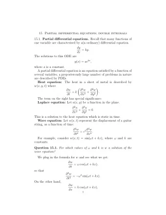
Symbolic solutions • Standard introductory differential equation courses focus on finding solutions analytically • Linear ODEs can be solved by integral transforms • Use DSolve[eqn,x,t] in Mathematica Differential equation: ˙ x ( t ) = − kx ( t ) Solution: x ( t ) = e − kt
Numerical solutions • In this class, we will be concerned with numerical solutions • Derivative function f is regarded as a black box • Given a numerical value x and t , the black box will return the time derivative of x
Physics-based simulation x i Newtonian laws gravity wind gust x i +1 elastic force . integrator . x i . x i +1 = x i + ∆ x ∆ x
• Overview of differential equation • Initial value problem • Explicit numeric methods • Implicit numeric methods • Modular implementation
Initial value problems In a canonical initial value problem, the behavior of the system is described by an ODE and its initial condition: x = f ( x, t ) ˙ x ( t 0 ) = x 0 To solve x ( t ) numerically, we start out from x 0 and follow the changes defined by f thereafter
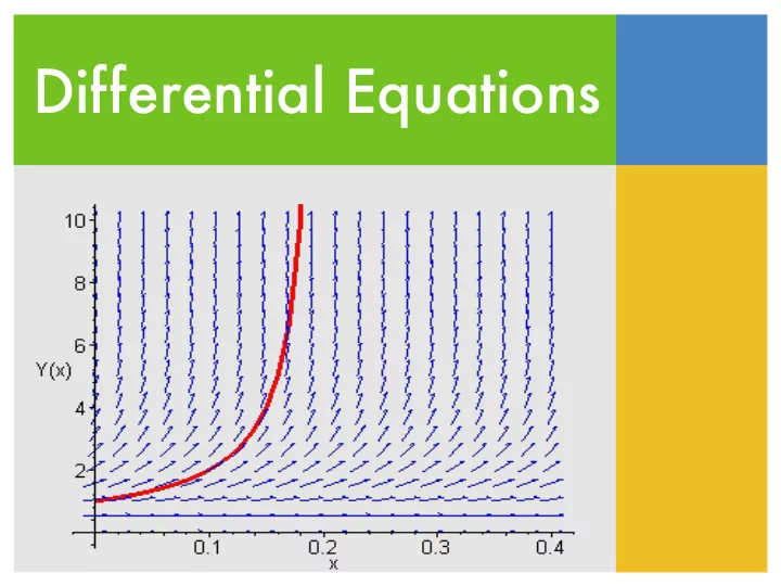
Vector field x 2 The differential equation can be visualized as a vector field x = f ( x , t ) ˙ x 1
Vector field x 2 The differential equation can be visualized as a vector field x = f ( x , t ) ˙ How does the vector field look like if f depends directly on time? x 1
Integral curves � f ( x , t ) dt t 0 f ( x , t )
Physics-based simulation x i Newtonian laws gravity wind gust x i +1 elastic force . integrator . x i . x i +1 = x i + ∆ x ∆ x
• Overview of differential equation • Initial value problem • Explicit numeric methods • Implicit numeric methods • Modular implementation
Explicit Euler method How do we get to the next state from the current state? x ( t 0 + h ) = x 0 + h ˙ x ( t 0 ) x ( t 0 + h ) Instead of following real integral x ( t 0 ) curve, p follows a polygonal path p Discrete time step h determines the errors
Problems of Euler method Inaccuracy The circle turns into a spiral no matter how small the step size is
Problems of Euler method Instability x = − k x ˙ x ( t ) = e − kt Symbolic solution: Oscillation: Divergence: How small the step size has to be?
Accuracy of Euler method • At each step, x ( t ) can be written in the form of Taylor series is a representation of a function as Taylor series: an infinite sum of terms calculated using the x ( t 0 ) + h 2 x ( t 0 ) + h 3 3! x (3) ( t 0 ) + . . . h n ∂ n x x ( t 0 + h ) = x ( t 0 ) + h ˙ 2! ¨ derivatives at a particular point n ! ∂ t n • What is the order of the error term in Euler method? • The cost per step is determined by the number of evaluations per step
Stability of Euler method • Assume the derivative function is linear d dt x = Ax • Look at x parallel to the largest eigenvector of A d dt x = λ x • Note that eigenvalue can be complex λ
The test equation • Test equation advances x by x n +1 = x n + h λ x n • Solving gives x n = (1 + h λ ) n x 0 • Condition of stability | 1 + h λ | ≤ 1
Stability region • Plot all the values of h λ on the complex plane where Euler method is stable
Real eigenvalue • If eigenvalue is real and negative, what kind of the motion does x correspond to? • a damping motion smoothly coming to a halt • The threshold of time step h ≤ 2 | λ | • What about the imaginary axis?
Imaginary eigenvalue • If eigenvalue is pure imaginary, Euler method is unconditionally unstable • What motion does x look like if the eigenvalue is pure imaginary? • an oscillatory or circular motion • We need to look at other methods
The midpoint method 1. Compute an Euler step ∆ x = hf ( x ( t 0 )) 2. Evaluate f at the midpoint f mid = f ( x ( t 0 ) + ∆ x 2 ) 3. Take a step using f mid x ( t 0 + h ) = x ( t 0 ) + hf mid x ( t + h ) = x 0 + hf ( x 0 + h 2 f ( x 0 ))
Accuracy of midpoint Prove that the midpoint method is correct within O( h 3 ) x ( t + h ) = x 0 + hf ( x 0 + h 2 f ( x 0 )) ∆ x = h 2 f ( x 0 ) f ( x 0 + ∆ x ) = f ( x 0 ) + ∆ x ∂ f ( x 0 ) + O ( x 2 ) ∂ x x ( t + h ) = x 0 + hf ( x 0 ) + h 2 2 f ( x 0 ) ∂ f ( x 0 ) + hO ( x 2 ) ∂ x x 0 + h 2 x 0 + O ( h 3 ) x ( t + h ) = x 0 + h ˙ 2 ¨
Stability region 2 = x n + h λ ( x n + 1 x n +1 = x n + h λ x n + 1 2 h λ x n ) x n +1 = x n (1 + h λ + 1 2( h λ ) 2 ) h λ = x + iy � 1 � x � x 2 − y 2 � �� � � + 1 � � + � ≤ 1 � � 0 2 xy 2 y � 1 + x + x 2 − y 2 � �� � � � � ≤ 1 2 � � y + xy �
Stability of midpoint • Midpoint method has larger stability region, but still unstable on the imaginary axis
Runge-Kutta method • Runge-Kutta is a numeric method of integrating ODEs by evaluating the derivatives at a few locations to cancel out lower-order error terms • Also an explicit method: x n + 1 is an explicit function of x n
Runge-Kutta method • q -stage p -order Runge-Kutta evaluates the derivative function q times in each iteration and its approximation of the next state is correct within O( h p+1 ) • What order of Runge-Kutta does midpoint method correspond to?
4-stage 4 th order Runge-Kutta = hf ( x 0 , t 0 ) k 1 hf ( x 0 + k 1 2 , t 0 + h = 2 ) k 2 hf ( x 0 + k 2 2 , t 0 + h = 2 ) k 3 = hf ( x 0 + k 3 , t 0 + h ) k 4 x 0 + 1 6 k 1 + 1 3 k 2 + 1 3 k 3 + 1 x ( t 0 + h ) = 6 k 4 x 0 f ( x 0 , t 0 ) 1 . f ( x 0 + k 1 2 , t 0 + h 2 ) 2 . f ( x 0 + k 2 2 , t 0 + h x 2 ) 3 . x ( t 0 + h ) f ( x 0 + k 3 , t 0 + h ) 4 . t
High order Runge-Kutta • RK3 and up are include part of the imaginary axis
Stage vs. order p 1 2 3 4 5 6 7 8 9 10 q min (p) 1 2 3 4 6 7 9 11 12-17 13-17 The minimum number of stages necessary for an explicit method to attain order p is still an open problem Why is fourth order the most popular Runge Kutta method?
Adaptive step size • Ideally, we want to choose h as large as possible, but not so large as to give us big error or instability • We can vary h as we march forward in time • Step doubling • Embedding estimate • Variable step, variable order
Step doubling Estimate by taking a full Euler step x a x a = x 0 + hf ( x 0 , t 0 ) Estimate by taking two half Euler steps x b e x temp = x 0 + h 2 f ( x 0 , t 0 ) x b = x temp + h 2 f ( x temp , t 0 + h 2 ) e = | x a − x b | is bound by O ( h 2 ) � � � 1 2 h Given error tolerance , what is the optimal step size? � e
Embedding estimate • Also called Runge-Kutta-Fehlberg • Compare two estimates of x ( t 0 + h ) • Fifth order Runge-Kutta with 6 stages • Forth order Runge-Kutta with 6 stages
Variable step, variable order • Change between methods of different order as well as step based on obtained error estimates • These methods are currently the last work in numerical integration
Problems of explicit methods • Do not work well with stiff ODEs • Simulation blows up if the step size is too big • Simulation progresses slowly if the step size is too small
Example: a bead on the wire y ( t ) Y ( t ) = ( x ( t ) , y ( t )) � x ( t ) � − x ( t ) � � Y = d ˙ = y ( t ) − ky ( t ) dt x ( t ) Explicit Euler’s method: � x ( t ) � − x ( t ) � � Y new = Y 0 + h ˙ Y ( t 0 ) = + h y ( t ) − ky ( t ) � (1 − h ) x ( t ) � Y new = (1 − kh ) y ( t )
Stiff equations • Stiffness constant: k • Step size is limited by the largest k • Systems that has some big k’s mixed in are called “stiff system”
• Overview of differential equation • Initial value problem • Explicit numeric methods • Implicit numeric methods • Modular implementation
Implicit methods Explicit Euler: Y new = Y 0 + hf ( Y 0 ) Implicit Euler: Y new = Y 0 + hf ( Y new ) Solving for such that � , at time , points t 0 + h f Y new directly back at �� � Y 0
Recommend


![CS475/CS675 Lecture 1: May 3, 2016 Basic Theory of Linear Algebra Reading: [TB] chapt 1 (p.](https://c.sambuz.com/1030692/cs475-cs675-lecture-1-may-3-2016-s.webp)


More recommend
Explore More Topics
Stay informed with curated content and fresh updates.