Deriving SGD for Neural Networks Swarthmore College CS63 Spring 2018 - PDF document

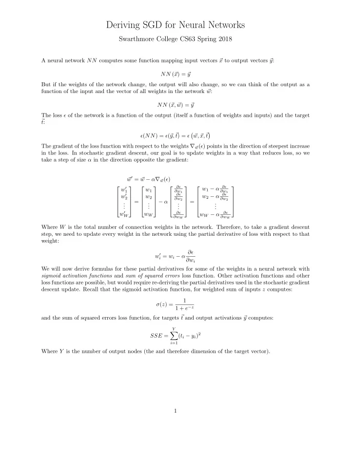
Deriving SGD for Neural Networks Swarthmore College CS63 Spring 2018 A neural network NN computes some function mapping input vectors � x to output vectors � y : NN ( � x ) = � y But if the weights of the network change, the output will also change, so we can think of the output as a function of the input and the vector of all weights in the network � w : NN ( � x, � w ) = � y The loss ǫ of the network is a function of the output (itself a function of weights and inputs) and the target � t : y,� x,� � � ǫ ( NN ) = ǫ ( � t ) = ǫ w, � � t The gradient of the loss function with respect to the weights ∇ � w ( ǫ ) points in the direction of steepest increase in the loss. In stochastic gradient descent, our goal is to update weights in a way that reduces loss, so we take a step of size α in the direction opposite the gradient: w ′ = � � w − α ∇ � w ( ǫ ) ∂ǫ w 1 − α ∂ǫ w ′         w 1 1 ∂w 1 ∂w 1 w ′ ∂ǫ w 2 − α ∂ǫ w 2 2      ∂w 2   ∂w 2   =  − α  = . .      .   .  . . . .         . . . .      w ′ w W ∂ǫ ∂ǫ w W − α W ∂w W ∂w W Where W is the total number of connection weights in the network. Therefore, to take a gradient descent step, we need to update every weight in the network using the partial derivative of loss with respect to that weight: i = w i − α ∂ǫ w ′ ∂w i We will now derive formulas for these partial derivatives for some of the weights in a neural network with sigmoid activation functions and sum of squared errors loss function. Other activation functions and other loss functions are possible, but would require re-deriving the partial derivatives used in the stochastic gradient descent update. Recall that the sigmoid activation function, for weighted sum of inputs z computes: 1 σ ( z ) = 1 + e − z and the sum of squared errors loss function, for targets � t and output activations � y computes: Y � ( t i − y i ) 2 SSE = i =1 Where Y is the number of output nodes (the and therefore dimension of the target vector). 1

Consider the following partially-specified neural network. We will find the partial derivative of the loss function with respect to one output-layer weight w o and one hidden layer weight w h . It should then be clear how these derivations extrapolate to the updates in the backpropagation algorithm we are implementing. · · · w h w o t 1 a i 1 a h 1 y 1 . . . w h � w o 1 � . . . . . . a i � � a h � y · · · w o Y � t 2 y Y First consider w o , the weight of an incoming edge for an output layer node. We want to compute the partial derivative of the loss function with respect to this weight: � Y � ∂ǫ ∂ � ( t i − y i ) 2 = ∂w o ∂w o i =1 Y ∂ � ( t i − y i ) 2 = ∂w o i =1 Since the only term in this sum that depends on w o is y 1 (the activation of the destination node for the edge with weight w o ), this derivative simplifies to: ∂ǫ ∂ ( t 1 − y 1 ) 2 = ∂w o ∂w o Here we can apply the chain rule [ f ( g ( x ))] ′ = f ′ ( g ( x )) g ′ ( x ) to get ∂ǫ = 2( t 1 − y 1 ) ∂ ( t 1 − y 1 ) ∂w o ∂w o = − 2( t 1 − y 1 ) ∂ ( y 1 ) ∂w o = − 2( t 1 − y 1 ) ∂ σ ( � w o 1 · � a h ) ∂w o Where the second step eliminated t 1 because it doesn’t depend on w o and thus has derivative 0, and the third step expanded y 1 to show the sigmoid activation function applied to the weighted sum of previous-layer inputs. We should now take a moment to find the derivative of a sigmoid function σ ′ ( z ), using the reciprocal rule [1 /f ] ′ = − f ′ /f 2 . 2

1 σ ( z ) = 1 + e − z e − z σ ′ ( z ) = (1 + e − z ) 2 = 1 + e − z − 1 (1 + e − z ) 2 � 1 + e − z � 1 1 = 1 + e − z − 1 + e − z 1 + e − z � � 1 1 = 1 − 1 + e − z 1 + e − z = σ ( z )(1 − σ ( z )) Now we can return to our partial derivative calculation and apply the chain rule in equation 1 to the sigmoid activation function: ∂ǫ = − 2( t 1 − y 1 ) ∂ σ ( � w o 1 · � a h ) ∂w o ∂w o � ∂ � = − 2( t 1 − y 1 ) σ ( � w o 1 · � a h )(1 − σ ( � w o 1 · � a h )) ( � w o 1 · � a h ) (1) ∂w o � ∂ � = − 2( t 1 − y 1 ) y 1 (1 − y 1 ) ( � w o 1 · � a h ) (2) ∂w o   | � a h |  ∂ � = − 2( t 1 − y 1 ) y 1 (1 − y 1 ) w i a i (3)  ∂w o i =1 � ∂ � = − 2( t 1 − y 1 ) y 1 (1 − y 1 ) w o a h 1 (4) ∂w o = − 2( t 1 − y 1 ) y 1 (1 − y 1 ) a h 1 (5) Where equation 2 follows from simplifying the sigmoid functions using the stored node activation y 1 , equa- tion 3 re-writes the dot product as a weighted sum, equation 4 eliminates the elements of the sum that don’t depend on w o , and equation 5 finalizes the partial derivative. Note that most of equation 5 depends only on the target and the output, and is therefore the same for all incoming edges to output node y 1 . We define δ o for output node o accordingly: δ 1 = y 1 (1 − y o )( t o − y o ) and the gradient descent update for weights w i from node i into an output node is then: w ′ i = w i − α ( − 2) δ o a i = w i + αδ o a i Where in the second equation, we’ve absorbed the constant 2 into the learning rate α . Next, consider w h , the weight of an incoming edge for a hidden layer node. Again, we want to compute the partial derivative of the loss function with respect to this weight: 3

� Y � ∂ǫ ∂ � ( t i − y i ) 2 = ∂w h ∂w h i =1 Y ∂ � ( t i − y i ) 2 = ∂w o i =1 This time, we have to consider each term in the sum, since the output of the hidden layer node can contribute to errors at every output node, so the weight of an edge into the hidden node can also affect every term. Luckily, each term in the sum is independent, so we will focus on the derivate of one representative term and reconstruct the full sum afterwards. Taking y 1 as our representative, we want to find: ∂ ( t 1 − y 1 ) 2 = 2( t 1 − y 1 ) ∂ ( t 1 − y 1 ) ∂w h ∂w h = − 2( t 1 − y 1 ) ∂ ( y 1 ) ∂w h = − 2( t 1 − y 1 ) ∂ σ ( � w o 1 · � a h ) ∂w h � ∂ � = − 2( t 1 − y 1 ) σ ( � w o 1 · � a h )(1 − σ ( � w o 1 · � a h )) ( � w o 1 · � a h ) ∂w h � ∂ � = − 2( t 1 − y 1 ) y 1 (1 − y 1 ) ( � w o 1 · � a h ) ∂w h   | � a h |  ∂ � = − 2( t 1 − y 1 ) y 1 (1 − y 1 ) w i a i  ∂w h i =1 The derivation so far has followed exactly the same procedure as equations 1–3 above, only that the partial derivative is with respect to w h instead of w o . This sum over � a h includes all of the activations in the last hidden layer, but only one of these activations depends on w h , so again we can simplify to � ∂ ∂ � ( t 1 − y 1 ) 2 = − 2( t 1 − y 1 ) y 1 (1 − y 1 ) ( w o a h 1 ) ∂w h ∂w h but now a h 1 depends on w h , so we need to break it down further: � ∂ � ∂ ( t 1 − y 1 ) 2 = − 2( t 1 − y 1 ) y 1 (1 − y 1 ) w o ( a h 1 ) (6) ∂w h ∂w h � ∂ � = − 2( t 1 − y 1 ) y 1 (1 − y 1 ) w o σ ( � a i · � w h ) (7) ∂w h � ∂ � = − 2( t 1 − y 1 ) y 1 (1 − y 1 ) w o σ ( � a i · � w h )(1 − σ ( � a i · � w h )) ( � a i · � w h ) ∂w h � ∂ � = − 2( t 1 − y 1 ) y 1 (1 − y 1 ) w o a h 1 (1 − a h 1 ) ( � a i · � w h ) ∂w h Equation 6 pulls out the w o term which does not depend on w h . Equation 7 breaks apart the activation of the hidden node, showing its dependence on weights and activations from the previous layer. The remaining equations follow similar steps to those from before, but this time applied to the activation function of the 4