Derivatives II: More about options Corporate Finance and Incentives - PowerPoint PPT Presentation
Derivatives II: More about options Corporate Finance and Incentives Lars Jul Overby Department of Economics University of Copenhagen October 2010 Lars Jul Overby (D of Economics - UoC) Derivatives II: More about options 10/10 1 / 22
Derivatives II: More about options Corporate Finance and Incentives Lars Jul Overby Department of Economics University of Copenhagen October 2010 Lars Jul Overby (D of Economics - UoC) Derivatives II: More about options 10/10 1 / 22
Generalization Let the initial stock price be S 0 and the current price of an option on the stock V . The expiration date of the option is T . During the life of the option, the stock can either move up to a new price of S 0 u or down to S 0 d ( u > 1; d < 1 ) . If the stock moves up, let the payoff from the option be V u . If the stock moves down, let the payoff from the option be V d . The value of the portfolio (long ∆ stocks and short 1 option) at expiration will be S 0 u ∆ − V u if the stock moves up. And S 0 d ∆ − V d if the stock moves down. Lars Jul Overby (D of Economics - UoC) 10/10 2 / 22
These will be equal when V u − V d ∆ = S 0 u − S 0 d When delta takes on this value, the portfolio is riskless and must earn the risk-free interest rate. At time 0 the value of the portfolio is therefore ( S 0 u ∆ − V u ) ( 1 + r f ) − T The initial cost of the portfolio is S 0 ∆ − V Lars Jul Overby (D of Economics - UoC) 10/10 3 / 22
Hence ( S 0 u ∆ − V u ) ( 1 + r f ) − T = S 0 ∆ − V S 0 ∆ − ( S 0 u ∆ − V u ) ( 1 + r f ) − T = V V u − V d = S 0 S 0 u − S 0 d � � S 0 u V u − V d ( 1 + r f ) − T S 0 u − S 0 d − V u − ( 1 + r f ) − T [ qV u + ( 1 − q ) V d ] = ( 1 + r f ) T − d q = u − d we can interpret q as the probability of an up movement in the stock and 1 − q as the probability of a down movement. The value of the option today is then the expected future value discounted at the risk-free rate. Lars Jul Overby (D of Economics - UoC) 10/10 4 / 22
Irrelevance of the stocks expected return The option pricing formula does not involve the probabilities of the stock price moving up or down. We are not valuing the option in absolute terms, but in terms of the price of the underlying stock. The probabilities of future up and down movements in the stock are already incorporated in the stock price no need to account for this again Lars Jul Overby (D of Economics - UoC) 10/10 5 / 22
Risk-neutral valuation The expected return on the stock, when q is assumed to be the probability of an up movement E ( S T ) = qS 0 u + ( 1 − q ) S 0 d = qS 0 ( u − d ) + S 0 d ( 1 + r f ) T − d = S 0 ( u − d ) + S 0 d u − d S 0 ( 1 + r f ) T = Setting the probability of an up movement in the stock to q is thus equivalent to the rate of return on the stock being the risk-free rate. This thus assumes that individuals are indifferent to risk - a risk-neutral world. Using the above q measure is an example of risk-neutral valuation. Lars Jul Overby (D of Economics - UoC) 10/10 6 / 22
Determining u and d How do we determine the size of the possible up and down movements in the stock. If It can be shown that these depend on the standard deviation or volatility of the stock return σ in the following manner √ h 1 + upside change = u = e σ d = 1 1 + downside change = u where h is the time interval, as a fraction of a year, over which the movement is observed (assuming σ is the annual volatility rate). In our example u = 80 60 = 1.3333 Thus we have an annualized volatility of the stock of e σ √ 2 = 1.3333 3 ln ( 1.3333 ) = = 0.3523 σ � 2 3 Lars Jul Overby (D of Economics - UoC) 10/10 7 / 22
Generalized binomial model For the binomial model to be in any way useful, there must be more than one period, since a stock price can take on more than 2 values However, adding more states with just a single time period is problematic, since it makes the market incomplete, meaning that finding unique derivatives prices is impossible we can’t create replicating portfolios Instead, we add more time periods to the model slice up the life of the option into smaller periods Lars Jul Overby (D of Economics - UoC) 10/10 8 / 22
Generalized binomial model Instead of assuming two possible stock price outcomes in 8 months, assume there are two time steps over the 8 month period. At each node at each time step, there are two possible stock price moves. This does not change the valuation method, but requires rebalancing of the replicating portfolio along the way. Dynamically adjusted portfolios - the delta changes The principle can be extended to a finer and finer division of the time period over which the option runs increasing the number of possible stock prices at expiration - until we reach the point where stock prices change continuously When valuing the option we use backwards induction Lars Jul Overby (D of Economics - UoC) 10/10 9 / 22
Two-stage binomial model Stock: S 0 = $ 60, σ = 35.23% Put option: K = $ 60, T = 2 / 3 r f = 1.5% p . a . Value option by two-stage binomial model u 4 = e 0.3523 ∗ √ 1 3 = 1.2256 1 + upside change (4 months) = d 4 = 1 1 + downside change (4 months) = = 0.8159 u 4 1 p = ( 1 + r f ) h − d = ( 1 + 0.015 ) 3 − 0.8159 = 0.4615 u − d 1.2256 − 0.8159 Lars Jul Overby (D of Economics - UoC) 10/10 10 / 22
Stock price and option development = S 0 $ 60 = $ 60 ∗ 1.2256 = $ 73.54 S 4, u = $ 60 ∗ 0.8159 = $ 48.95 S 4, d = $ 60 ∗ 1.2256 ∗ 1.2256 = $ 90.13 S 8, u , u S 8, u , d = S 8, d , u = $ 60 ∗ 1.2256 ∗ 0.8159 = $ 60.00 = $ 60 ∗ 0.8159 ∗ 0.8159 = $ 39.94 S 8, d , d = V u , u = $ 0 p 8, u , u p 8, u , d = V u , d = $ 0 = V d , d = $ 60 − $ 39.94 = $ 20.06 p 8, d , d Lars Jul Overby (D of Economics - UoC) 10/10 11 / 22
Option value at month 4 Option delta = 0 − 20.06 60 − 39.94 = − 1 Construct a leveraged position in delta shares which gives an identical payoff to the option: S 8, d , d S 8, d , u Sell 1 share − $ 39.94 − $ 60.00 Invest PV of $ 60 $ 60.00 $ 60.00 Total payoff $ 20.06 $ 0 Value of put in month 4: put 4, d = − $ 48.95 + $ 60 ∗ ( 1 + 0.015 ) − 1 3 = $ 10.75 or put 4, d = ( 1 + r f ) − h [ pV u , d + ( 1 − p ) V d , d ] = ( 1 + 0.015 ) − 1 3 [ 0.4615 ∗ $ 0 + ( 1 − 0.4615 ) ∗ $ 20.06 ] = $ 10.75 Lars Jul Overby (D of Economics - UoC) 10/10 12 / 22
Option value now 0 − 10.75 Option delta = 73.54 − 48.95 = − 0.437 Construct a leveraged position in delta shares which gives an identical payoff to the option: S 4, d S 4, u Sell 0.437 shares − $ 21.39 − $ 32.14 Invest PV of $ 32.14 $ 32.14 $ 32.14 Total payoff $ 10.75 $ 0 Value of put now: put = − $ 60 ∗ 0.437 + $ 32.14 ∗ ( 1 + 0.015 ) − 1 3 = $ 5.76 or put = ( 1 + 0.015 ) − 1 3 [ 0.4616 ∗ $ 0 + ( 1 − 0.4616 ) ∗ $ 10.75 ] = $ 5.76 Lars Jul Overby (D of Economics - UoC) 10/10 13 / 22
Generalized binomial model Two step ( 1 + r f ) − h [ qV u , u + ( 1 − q ) V u , d ] V u = ( 1 + r f ) − h [ qV u , d + ( 1 − q ) V d , d ] V d = ( 1 + r f ) − h [ qV u + ( 1 − q ) V d ] = V q 2 V u , u + 2 q ( 1 − q ) V u , d + ( 1 − q ) 2 V dd ( 1 + r f ) − 2 h � � = V Generalized to N-steps - see formula 8.2 in book ( π = q ) Lars Jul Overby (D of Economics - UoC) 10/10 14 / 22
The Black-Scholes Model (1973) Assume we take the binomial model to the limit, and divide the options life into an infinite number of subperiods. This gives us continuously adjusting stock prices which we assume to be lognormally distributed. The principle of option evaluation is still the same as in the simple binomial models, but we now have to rebalance the replicating portfolio continuously. Lars Jul Overby (D of Economics - UoC) 10/10 15 / 22
The Black-Scholes Model Most critical assumptions: Underlying asset price follows a continuous time diffusion (no jumps) Volatility is constant and known Returns are lognormally distributed Markets are frictionless Lars Jul Overby (D of Economics - UoC) 10/10 16 / 22
The Black-Scholes model provides a relatively simple way to handle this continuous rebalancing and value options in such a setup. Value of an option: SN ( d 1 ) − Ke − r f t N ( d 2 ) = call Ke − r f t N ( − d 2 ) − SN ( − d 1 ) = put r f + σ 2 / 2 ln ( S / K ) + � � t d 1 = σ √ t √ = d 2 d 1 − σ t N ( d ) = cumulative normal probability density function = S stock price now = exercise price of option K t = number of periods to exercise date = standard deviation (volatility) per period of stock return σ r f = interest rate per period Lars Jul Overby (D of Economics - UoC) 10/10 17 / 22
Stock: S 0 = $ 60, σ = 35.23% Put option: K = $ 60, T = 2 / 3 r f = 1.5% p . a . continuously compounded Black-Scholes formula for a put Ke − r f t N ( − d 2 ) − SN ( − d 1 ) = put r f + σ 2 / 2 ln ( S / K ) + � � t = d 1 σ √ t 0.015 + 0.3523 2 / 2 ln ( 60 / 60 ) + � � 2 / 3 = 0.3523 √ 2 / 3 = 0.1786 √ √ d 2 = d 1 − σ t = 0.1786 − 0.3523 2 / 3 = − 0.1091 N ( − d 1 ) = 0.4291 N ( − d 2 ) = 0.5434 60 e − 0.015 ∗ 2 / 3 0.5434 − 60 ∗ 0.4291 = 6.534 = put Lars Jul Overby (D of Economics - UoC) 10/10 18 / 22
As the number of intervals used in the binomial model increases, the option price converges towards the option price from the Black-Scholes model. The Black-Scholes formula is generally quicker and more accurate to use than the binomial model. However, there are a number of cases in which the Black-Scholes model cannot be applied. The Black-Scholes model cannot handle early exercise. Lars Jul Overby (D of Economics - UoC) 10/10 19 / 22
Recommend
More recommend
Explore More Topics
Stay informed with curated content and fresh updates.
