Demonstrative presentation of AIM/Impact model Mr. Kiyoshi - PowerPoint PPT Presentation
APEIS Capacity Building Workshop on Integrated Environmental Assessment in the Asia Pacific Region October 2002 Demonstrative presentation of AIM/Impact model Mr. Kiyoshi Takahashi, NIES, Japan Dr. Yasuaki Hijioka, NIES, Japan Dr. Amit Garg,
APEIS Capacity Building Workshop on Integrated Environmental Assessment in the Asia Pacific Region October 2002 Demonstrative presentation of AIM/Impact model Mr. Kiyoshi Takahashi, NIES, Japan Dr. Yasuaki Hijioka, NIES, Japan Dr. Amit Garg, Winrock International, India
Outputs of AIM/Impact -500 0 +500 ( kg/ha) Change of crop productivity 1990 2050 (mm/year) 3 30 300 0.3 Change of river discharge Water withdrawal
Objective of the course ● Introduction of standard procedures of impact assessment using AIM/Impact. ● Demonstration of specific procedures of assessment of potential crop productivity under anticipated climate change. – STEP1: Collection of input data – STEP2: Scenario development – STEP3: Parameter setting and simulation – STEP4: Display and analysis of the results ● Brief introduction of AIM/Impact [Country]
Standard work flow of impact assessment in AIM/Impact ● 1. Collection of input data and importing them into GIS database – GRASS GIS ● 2. Future scenario development – Interpolation – Simple climate model and Pattern scaling ● 3. Simulation – Parameter setting ● 4. Display and analysis of the results – Visualization – Aggregation – Feedback or higher impact
GRASS (Geographic Reseoucres Analysis Support System) ● Gegraphical Information System Software ● Run on unix oprating systems (Solaris, Linux, etc.) ● Advantage – Distributed on internet (Free) – Raster (gridded) data – Source codes available (C language) – Modules can be developed by users with the GRASS developers' library. ● Disadvantage – Unix – Inexcelent graphical user interface
Example of spatial data managed in GRASS GIS Obserbation climatology Population density Assessment results GCM results
Data collection ● Current climate – Monthly or daily mean climatology ● CRU/UEA LINK climatology (1901-1996, 0.5x0.5, monthly) ● GEWEX/NASA ISLSCP (1987 and 1988, 1.0x1.0, monthly, daily or 6-hourly) ● Future climate projection – Output of General Circulation Models (GCMs) ● IS92a simulations (IPCC-DDC) ● SRES simulations (IPCC-DDC) ● Simulation by CCSR/NIES – Output of Regional Climate Models (RCM) ● Not available yet
Data collection ● Soil – Chemical and physical character of soil ● FAO Soil Map of the World ● Landuse – Landuse classification derived from remote- sensing data ● 1km x 1km GLCC (EDC/EROS/USGS) ● Population – Gridded population density ● GPW2 (CIESIN/Colombia University, 2.5min) ● LandScan2000 (1km x 1km)
Climate scenario ● Future changes of climate (temperature, rain, radiation, wind etc.) are deduced from GCMs results distributed at IPCC-DDC or provided by NIES/CCSR. ● In order to compromise with the very low resolution of GCM results, the results of GCMs are interpolated and current observed climatology is used for expressing spatial detail. ● For assessing various future path of GHG emission, "pattern scaling method” is employed to develop climate scenario.
Pattern scaling GHG increase run (GCM) ― Minus Control run (GCM) = Spatial pattern of climate change (GCM) Spatial interpolation Scaling Interpolated and scaled ⊿T spatial pattern of CC + Various emission path Current climate (observed) t = Climate change scenario Simple climate model
Simulation ● Simulation models in AIM/Impact are Unix shell files which consist of GRASS commands originally developed using GRASS-GIS library and standard GRASS commands included in the GRASS distribution. ● Some models refer to the model parameter files for reading assumption or information other than spatial input data managed in GIS.
Models in AIM/Impact ● Water balance model – Penman PET – Thornthwaite PET – Surface runoff ● River discharge model ● Potential crop productivity model ● Water demand model ● Malaria potential model ● Vegetation classification model ● Vegetation move possibility model
Visualization and analysis ● Grasping spatial pattern of impact through visualization – Detection of critically damaged region – Time series analysis based on animation ● Spatial aggregation – Aggregation (spatial average) based on administrative boundaries – Time series trend – Linkage with the other assessment frameworks (ex. Economic model)
Demonstration of assessment of agricultural impact ● What will be done in the demonstration – Calculate potential crop productivity of rice and winter wheat in Asia. – Display some figures of the results focusing India. ● Objective – Demonstrate the procedure to assess climate change impact using AIM/Impact with going through simplified assessment processes step by step.
Procedure AIM/Impact GIS data archive (1) copygrassdata.sh Dataset for assessment in the workshop LINK historical NIES/CCSR Soil and surface Administrative observation GCM results field data boundaries (2) interpolation.sh Interpolated GCM results (3) scenariocreate.sh Climate scenario (4) rainfed.sh (5) nowaterstress.sh (6) createirigdata.sh Potential productivity Potential productivity of irrigated area Statistical data irrigated ratio Spatial data of under rain-fed agriculture under perfect irrigation (7) considerirrigation.sh Potential productivity considering irrigation (8) indiafigure.sh Figures of results
AIM/Impact GIS data archive (1) copygrassdata.sh Dataset for assessment in the workshop LINK historical NIES/CCSR Soil and surface Administrative observation GCM results field data boundaries (2) interpolation.sh Interpolated Interpolation GCM results (3) scenariocreate.sh Climate scenario (4) rainfed.sh (5) nowaterstress.sh (6) createirigdata.sh Potential productivity Potential productivity of irrigated area Statistical data under rain-fed agriculture irrigated ratio Spatial data of under perfect irrigation (interpolation.sh) (7) considerirrigation.sh Potential productivity considering irrigation (8) indiafigure.sh Figures of results NIES/CCSR GCM (5.6 x 5.6) Spline interpolation Monthly mean temperature in 0.5 x 0.5 2050s under IS92a scenrio.
AIM/Impact GIS data archive (1) copygrassdata.sh Dataset for assessment in the workshop LINK historical NIES/CCSR Soil and surface Administrative observation GCM results field data boundaries (2) interpolation.sh Interpolated Temperature scenario GCM results (3) scenariocreate.sh Climate scenario (4) rainfed.sh (5) nowaterstress.sh (6) createirigdata.sh Potential productivity Potential productivity of irrigated area Statistical data under rain-fed agriculture irrigated ratio Spatial data of under perfect irrigation (scenariocreate.sh) (7) considerirrigation.sh Potential productivity considering irrigation (8) indiafigure.sh Figures of results JAN FEB MAR JAN FEB MAR APR MAY JUN APR MAY JUN JUL AUG SEP JUL AUG SEP LINK historical temperature Temperature scenario (1961-1990) (2050s, CCSR/NIES model) OCT NOV DEC OCT NOV DEC -10 0 10 20 30 40 (C o )
AIM/Impact GIS data archive (1) copygrassdata.sh Dataset for assessment in the workshop LINK historical NIES/CCSR Soil and surface Administrative observation GCM results field data boundaries (2) interpolation.sh Interpolated Precipitation scenario GCM results (3) scenariocreate.sh Climate scenario (4) rainfed.sh (5) nowaterstress.sh (6) createirigdata.sh Potential productivity Potential productivity of irrigated area Statistical data under rain-fed agriculture irrigated ratio Spatial data of under perfect irrigation (scenariocreate.sh) (7) considerirrigation.sh Potential productivity considering irrigation (8) indiafigure.sh Figures of results JAN FEB MAR JAN FEB MAR APR MAY JUN APR MAY JUN JUL AUG SEP JUL AUG SEP LINK historical precipitation Precipitation scenario (1961-1990) (2050s, CCSR/NIES model) 1 100 200 300 (mm/month) OCT NOV DEC OCT NOV DEC
Example of parameter Characteristics of crop growth cropname WheatSC WheatWC Whitepotato PhaseolusbeanTEC PhaseolusbeanT RC Soybean Rice Cotton Sweetpotato Cassav a Pearlmillet SorghumT RC MaizeTRC SorghumT EC MaizeT EC crop_kind 1 1 1 1 2 2 2 2 2 2 3 3 3 4 4 m_gp 100 200 150 90 120 120 130 160 150 330 90 120 120 110 110 min_gp 90 90 90 50 50 75 80 150 90 180 55 90 70 90 70 m_lai 5 5 5 4 4 4 5 3 4.5 3 4 4 4 3 4 m_hi 0.4 0.4 0.6 0.3 0.3 0.35 0.3 0.07 0.55 0.55 0.25 0.25 0.35 0.25 0.35 bean 0 0 0 1 1 1 0 0 0 0 0 0 0 0 0 hi_kind 0 0 0 0 0 0 0 0 1 1 0 0 0 0 0 gp_kind 1 0 0 1 0 0 0 0 0 0 0 0 0 2 2 thres_l 5 5 7 7 7 13 12 15 10 10 15 15 12 15 12 thres_u 25 25 30 32 32 38 36 38 40 35 45 38 40 38 40
Recommend
More recommend
Explore More Topics
Stay informed with curated content and fresh updates.
