Decision Making under Uncertainty Part 1: Introduction to - PDF document

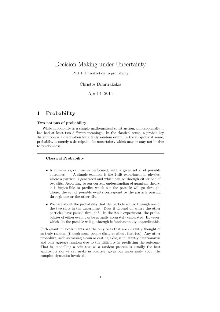
Decision Making under Uncertainty Part 1: Introduction to probability Christos Dimitrakakis April 4, 2014 1 Probability Two notions of probability While probability is a simple mathematical construction, philosophically it has had at least two different meanings. In the classical sense, a probability distribution is a description for a truly random event. In the subjectivist sense, probabilty is merely a description for uncertainty which may or may not be due to randomness. Classical Probability • A random experiment is performed, with a given set S of possible outcomes. A simple example is the 2-slit experiment in physics, where a particle is generated and which can go through either one of two slits. According to our current understanding of quantum theory, it is impossible to predict which slit the particle will go through. There, the set of possible events correspond to the particle passing through one or the other slit. • We care about the probability that the particle will go through one of the two slots in the experiment. Does it depend on where the other particles have passed through? In the 2-slit experiment, the proba- bilities of either event can be actually accurately calculated. However, which slit the particle will go through is fundamentally unpredictable. Such quantum experiments are the only ones that are currently thought of as truly random (though some people disagree about that too). Any other procedure, such as tossing a coin or casting a die, is inherently deterministic and only appears random due to the difficulty in predicting the outcome. That is, modelling a coin toss as a random process is usually the best approximation we can make in practice, given our uncertainty about the complex dynamics involved. 1

2 CS 709: 1. Introduction to probability Subjective Probability • We assume that S is a set of possible worlds or realities, This set can be quite large and include anything imaginable. For example, it may include worlds where dragons are real. However, in practice one only cares about certain aspects of the world. • We can interpret the probability of a world in S as a belief that it is the true world. In such a setting there is an actual true world ω ∗ ∈ S , which is simply unknown. This could have been set by Nature to an arbritrary value deter- ministically. The probability only reflects our lack of knowledge. 1.1 Sets, experiments and sample spaces Set theory definitions A very useful way to describe a set A is as follows A ≜ { x | x have property Y } for example B ( c, r ) ≜ { x ∈ R n | ∥ x − c ∥ ≤ r } describes the set of points enclosed in an n -dimensional sphere of radius r with center c ∈ R n . • If an element x belongs to a set A , we write x ∈ A . • Let the sample space S be a set such that x ∈ S always. • We say that A is a subset of B or that B contains A , and write A ⊂ B , iff, x ∈ B for any x ∈ A . • Let B \ A ≜ { x | x ∈ B ∧ x / ∈ A } be the set difference. • Let A △ B ≜ ( B \ A ) ∪ ( A \ B ) be the symmetric set difference. • The complement of any A ⊂ S is A ∁ ≜ S \ A . • The empty set is ∅ = S ∁ . • The union of n sets: A 1 , . . . , A n is ∪ n i =1 A i = A 1 ∪ · · · ∪ A n . • The intersection of n sets A 1 , . . . , A n is ∩ n i =1 A i = A 1 ∩ · · · ∩ A n . • A and B are disjoint if A ∩ B = ∅ . Experiments and sample spaces

CS 709: Decision Making under Uncertainty 3 Experiments The set of possible experimental outcomes of an experiment is called the sample space S . • S must contain all possible outcomes. • Each statistician i may consider a different S i for the same experiment. Example 1.1. Experiment: give medication to a patient. • S 1 = { Recovery within a day , No recovery after a day } . • S 2 = { The medication has side-effects , No side-effect } . • S 3 = all combinations of the above. Product spaces • We perform n experiments. • Assume that the i -th experiment has sample space S i . • The Cartesian product or product space is defined as S 1 × · · · × S n = { ( s 1 , . . . , s n ) | s i ∈ S i , ∀ i ∈ { 1 , . . . , n }} (1.1) the set of all ordered n -tuples ( s 1 , . . . , s n ). • The sample space ∏ n i =1 S i can be thought of as a sample space of a com- posite experiment in which all n experiments are performed. Identical experiment sample spaces • In many cases, S i = S for all i , i.e. the sample space is identical for all individual experiment (e.g. n coin tosses). • We then write S n = ∏ n i =1 S . 1.2 Events, measure and probability Events and probability Probability of a set If A is a subset of S , the probability of A is a measure of the chances that the outcome of the experiment will be an element of A .

4 CS 709: 1. Introduction to probability A B r r r r r r C r r r r r r Figure 1: A fashionable apartment Which sets? Ideally, we would like to be able to assign a probability to every subset of S . However, for technical reasons, this is not possible. Example 1.2. Let X be uniformly distributed on [0 , 1] . • What is the probability that X will be in [0 , 1 / 4) ? • What is the probability that X will be in [1 / 4 , 1] ? • What is the probability that X will be a rational number? Measure theory primer Imagine that you have an apartment S composed of three rooms, A, B, C . There are some coins on the floor and a 5-meter-long red carpet. We can measure various things in this apartment. Area • A: 4 × 5 = 20 m 2 . • B: 6 × 4 = 24 m 2 . • C: 2 × 5 = 10 m 2 . Coins on the floor • A: 3. • B: 4

CS 709: Decision Making under Uncertainty 5 • C: 5. Length of red carpet • A: 0 m • B: 0 . 5 m • C: 4 . 5 m . Measure the sets: F = {∅ , A, B, C, A ∪ B, A ∪ C, B ∪ C, A ∪ B ∪ C } . It is easy to see that the union of any sets in F is also in F . In other words, F is closed under union. Furthermore, F contains the whole space S . Note that all those measures have an additive property . Measure and probability As previously mentioned, the probability of A ⊂ S is a measure of the chances that the outcome of the experiment will be an element of A . Here we give a precise definition of what we mean by measure and probability. Definition 1.1 (A field on S ) . A family F of sets, such that for each A ∈ F , A ⊂ S , is called a field on S if and only if 1. S ∈ F 2. if A ∈ F , then A ∁ ∈ F . 3. For any A 1 , A 2 , . . . , A n such that A i ∈ F , it holds that: ∪ n i =1 A i ∈ F . From the above definition, it is easy to see that A i ∩ A j is also in the field. Definition 1.2 ( σ -field on S ) . A family F of sets, such that ∀ A ∈ F , A ⊂ S , is called a σ -field on S if and only if 1. S ∈ F 2. if A ∈ F , then A ∁ ∈ F . 3. For any sequence A 1 , A 2 , . . . such that A i ∈ F , it holds that: ∪ ∞ i =1 A i ∈ F . It is easy to verify that the F given in the apartment example satisfies these properties. Definition 1.3 (Measure) . A measure λ on ( S , F ) is a function λ : F → R + such that 1. λ ( ∅ ) = 0 . 2. λ ( A ) ≥ 0 for any A ∈ F .

6 CS 709: 1. Introduction to probability 3. For any collection of subsets A 1 , . . . , A n with A i ∈ F and A i ∩ A j = ∅ . ( ∞ ) ∞ ∪ ∑ λ A i = λ ( A i ) (1.2) i =1 i =1 It is easy to verify that the floor area, the number of coins, and the length of the red carpet are all measures. In fact, the area and length correspond to what is called a Lebesgue measure and the number of coins to a counting measure . Definition 1.4 (Probability measure) . A probability measure P on ( S , F ) is a function P : F → [0 , 1] such that: 1. P ( S ) = 1 2. P ( ∅ ) = 0 3. P ( A ) ≥ 0 for any A ∈ F . 4. If A 1 , A 2 , . . . are disjoint then ( ∞ ) ∞ ∪ ∑ P A i = P ( A i ) (union) i =1 i =1 ( S, F , P ) is called a probability space . So, probability is just a special type of measure. 1.2.1 The Lebesgue measure Definition 1.5 (Outer measure) . Let ( S , F , λ ) be a measure space. The outer measure of a set A ⊂ S is: λ ∗ ≜ inf A ⊂ ∪ ∑ B k λ ( B k ) . (1.3) k k Definition 1.6 (Inner measure) . Let ( S , F , λ ) be a measure space. The outer measure of a set A ⊂ S is: λ ∗ ≜ λ ( S ) − λ ( S \ A ) . (1.4) Definition 1.7 (Lebesgue measurable sets) . A set A is (Lebesgue) measurable if the outer and inner measures are equal. λ ∗ ( A ) = λ ∗ ( B ) . (1.5) The common value of the inner and outer measure is called the Lebesgue mea- sure 1 ¯ λ = λ ∗ ( A ) . 1 It is easy to see that ¯ λ is a measure.

CS 709: Decision Making under Uncertainty 7 w A S h B Figure 2: In the above case, S is a unit square and taking P to be the Lebesgue measure, we see that P ( S ) = 1 · 1, P ( A ) = 1 · w , P ( B ) = h · 1 and P ( A ∩ B ) = wh , so A and B are independent. 1.3 Conditioning and independence Independent events and conditional probability Events correspond to sets. Thus, the probability of the event that a draw from S is in A is equal to the probability measure of A , P ( A ). Definition 1.8 (Independent events) . Two events A, B are independent if P ( A ∩ B ) = P ( A ) P ( B ) . The events in a family F of events are independent if for any sequence A 1 , A 2 , . . . of events in F , ( n ) n ∩ ∏ P A i = P ( A i ) (independence) i =1 i =1 Definition 1.9 (Conditional probability) . The conditional probability of A when B , s.t. P ( B ) > 0 , is given is: P ( A | B ) ≜ P ( A ∩ B ) . (1.6) P ( B )