Decision Making Under First Application to . . . Uncertainty with - PowerPoint PPT Presentation

Decision Theory: A . . . Which Is the Optimal . . . Teaching . . . How to Speed Up . . . Decision Making Under First Application to . . . Uncertainty with 2nd Application to . . . Explaining . . . Applications to Geosciences Application to . . . Future Work Plans and Finance Home Page Laxman Bokati Title Page Computational Science Program ◭◭ ◮◮ University of Texas at El Paso El Paso, TX 79968, USA ◭ ◮ lbokati@miners.utep.edu Page 1 of 51 Go Back Full Screen Close Quit

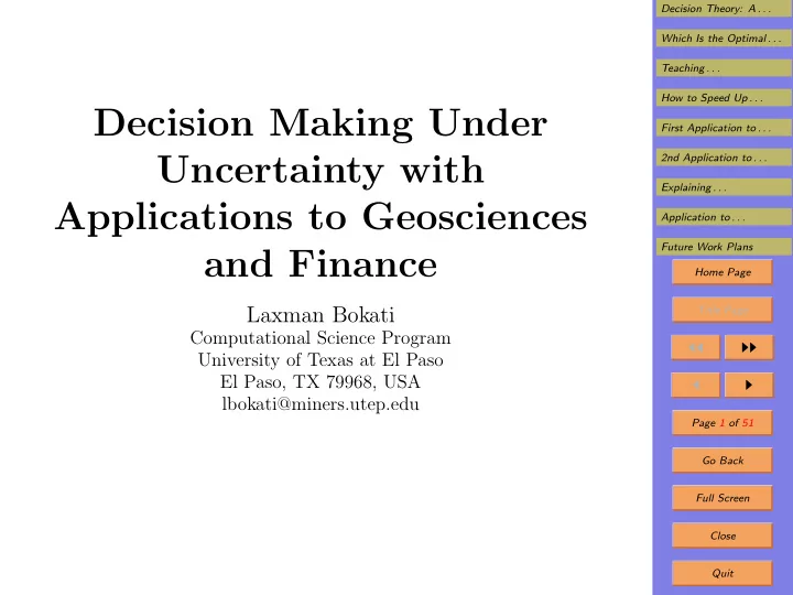
Decision Theory: A . . . Which Is the Optimal . . . 1. Outline Teaching . . . • Introduction How to Speed Up . . . First Application to . . . • Decision theory: a brief reminder 2nd Application to . . . • What is the optimal approximation family Explaining . . . • Teaching optimization Application to . . . Future Work Plans • How to speed up computations Home Page • Applications to finance: Title Page – is “no trade theorem” really a paradox ◭◭ ◮◮ – why buying and selling prices differ ◭ ◮ – explaining “telescoping effect” Page 2 of 51 • Application to geosciences Go Back • Future work plans Full Screen Close Quit

Decision Theory: A . . . Which Is the Optimal . . . 2. Formulation of the Problem Teaching . . . • In many practical situations, we need to make a deci- How to Speed Up . . . sion. First Application to . . . 2nd Application to . . . • In many applications, we do not know the exact con- Explaining . . . sequences of each action. Application to . . . • In such situations, we need to make a decision under Future Work Plans uncertainty. Home Page • In many application areas, uncertainty is small – and Title Page can be made even smaller by extra measurements. ◭◭ ◮◮ • For example, for a self-driving car, we can accurately ◭ ◮ measure all the related values and events. Page 3 of 51 • However, there are applications when it is difficult to Go Back decrease uncertainty. Full Screen • One such area is anything related to human activities. Close Quit

Decision Theory: A . . . Which Is the Optimal . . . 3. Formulation of the Problem (cont-d) Teaching . . . • Humans make individual decisions based on their per- How to Speed Up . . . ceived value of different alternatives. First Application to . . . 2nd Application to . . . • Such behavior affects economics and finance. Explaining . . . • So in economics and finance, it is important to make Application to . . . decision under uncertainty. Future Work Plans Home Page • Another area where it is difficult to decrease uncer- tainty is geosciences. Title Page • The only way to get a more accurate picture of what ◭◭ ◮◮ is going on beneath the earth surface is to dig a well. ◭ ◮ • But the whole purpose of decision making is to decide Page 4 of 51 whether such an expensive procedure is worth doing. Go Back • Decision making under under uncertainty and its ap- Full Screen plications is the main topic of my research. Close Quit

Decision Theory: A . . . Which Is the Optimal . . . 4. Decision Theory: A Brief Reminder Teaching . . . • To make a decision, we must: How to Speed Up . . . First Application to . . . – find out the user’s preference, and 2nd Application to . . . – help the user select an alternative which is the best Explaining . . . – according to these preferences. Application to . . . • Traditional approach is based on an assumption that Future Work Plans for each two alternatives A ′ and A ′′ , a user can tell: Home Page – whether the first alternative is better for him/her; Title Page we will denote this by A ′′ < A ′ ; ◭◭ ◮◮ – or the second alternative is better; we will denote ◭ ◮ this by A ′ < A ′′ ; Page 5 of 51 – or the two given alternatives are of equal value to the user; we will denote this by A ′ ∼ A ′′ . Go Back Full Screen Close Quit

Decision Theory: A . . . Which Is the Optimal . . . 5. The Notion of Utility Teaching . . . • Under the above assumption, we can form a natural How to Speed Up . . . numerical scale for describing preferences. First Application to . . . 2nd Application to . . . • Let us select a very bad alternative A 0 and a very good Explaining . . . alternative A 1 . Application to . . . • Then, most other alternatives are better than A 0 but Future Work Plans worse than A 1 . Home Page • For every prob. p ∈ [0 , 1], we can form a lottery L ( p ) Title Page in which we get A 1 w/prob. p and A 0 w/prob. 1 − p . ◭◭ ◮◮ • When p = 0, this lottery simply coincides with the ◭ ◮ alternative A 0 : L (0) = A 0 . Page 6 of 51 • The larger the probability p of the positive outcome Go Back increases, the better the result: Full Screen p ′ < p ′′ implies L ( p ′ ) < L ( p ′′ ) . Close Quit

Decision Theory: A . . . Which Is the Optimal . . . 6. The Notion of Utility (cont-d) Teaching . . . • Finally, for p = 1, the lottery coincides with the alter- How to Speed Up . . . native A 1 : L (1) = A 1 . First Application to . . . 2nd Application to . . . • Thus, we have a continuous scale of alternatives L ( p ) Explaining . . . that monotonically goes from L (0) = A 0 to L (1) = A 1 . Application to . . . • Due to monotonicity, when p increases, we first have Future Work Plans L ( p ) < A , then we have L ( p ) > A . Home Page • The threshold value is called the utility of the alterna- Title Page tive A : ◭◭ ◮◮ def u ( A ) = sup { p : L ( p ) < A } = inf { p : L ( p ) > A } . ◭ ◮ • Then, for every ε > 0, we have Page 7 of 51 L ( u ( A ) − ε ) < A < L ( u ( A ) + ε ) . Go Back • We will describe such (almost) equivalence by ≡ , i.e., Full Screen we will write that A ≡ L ( u ( A )). Close Quit

Decision Theory: A . . . Which Is the Optimal . . . 7. A Rational Agent Should Maximize Utility Teaching . . . • Suppose that we have found the utilities u ( A ′ ), u ( A ′′ ), How to Speed Up . . . . . . , of the alternatives A ′ , A ′′ , . . . First Application to . . . 2nd Application to . . . • Which of these alternatives should we choose? Explaining . . . • By definition of utility, we have: Application to . . . • A ≡ L ( u ( A )) for every alternative A , and Future Work Plans • L ( p ′ ) < L ( p ′′ ) if and only if p ′ < p ′′ . Home Page Title Page • We can thus conclude that A ′ is preferable to A ′′ if and only if u ( A ′ ) > u ( A ′′ ). ◭◭ ◮◮ ◭ ◮ • In other words, we should always select an alternative with the largest possible value of utility. Page 8 of 51 Go Back Full Screen Close Quit

Decision Theory: A . . . Which Is the Optimal . . . 8. How to Estimate Utility of an Action Teaching . . . • For each action, we usually know possible outcomes How to Speed Up . . . First Application to . . . S 1 , . . . , S n . 2nd Application to . . . • We can often estimate the prob. p 1 , . . . , p n of these out- Explaining . . . comes. Application to . . . • By definition of utility, each situation S i is equiv. to a Future Work Plans lottery L ( u ( S i )) in which we get: Home Page • A 1 with probability u ( S i ) and Title Page • A 0 with the remaining probability 1 − u ( S i ). ◭◭ ◮◮ • Thus, the action is equivalent to a complex lottery in ◭ ◮ which: Page 9 of 51 • first, we select one of the situations S i with proba- Go Back bility p i : P ( S i ) = p i ; Full Screen • then, depending on S i , we get A 1 with probability P ( A 1 | S i ) = u ( S i ) and A 0 w/probability 1 − u ( S i ). Close Quit

Decision Theory: A . . . Which Is the Optimal . . . 9. How to Estimate Utility of an Action (cont-d) Teaching . . . • Reminder: How to Speed Up . . . First Application to . . . • first, we select one of the situations S i with proba- 2nd Application to . . . bility p i : P ( S i ) = p i ; Explaining . . . • then, depending on S i , we get A 1 with probability Application to . . . P ( A 1 | S i ) = u ( S i ) and A 0 w/probability 1 − u ( S i ). Future Work Plans • The prob. of getting A 1 in this complex lottery is: Home Page n n � � Title Page P ( A 1 ) = P ( A 1 | S i ) · P ( S i ) = u ( S i ) · p i . i =1 i =1 ◭◭ ◮◮ • In the complex lottery, we get: ◭ ◮ � n • A 1 with prob. u = p i · u ( S i ), and Page 10 of 51 i =1 Go Back • A 0 w/prob. 1 − u . Full Screen • So, we should select the action with the largest value of expected utility u = � p i · u ( S i ). Close Quit

Decision Theory: A . . . Which Is the Optimal . . . 10. To Practical Applications of Decision Theory Teaching . . . • The numerical value of utility depends on the selection How to Speed Up . . . of the alternatives A 0 and A 1 . First Application to . . . 2nd Application to . . . • If we select a different pair ( A ′ 0 , A ′ 1 ), then utility changes Explaining . . . into u ′ ( A ) = a · u ( A ) + b for some a > 0 and b . Application to . . . • The dependence of utility of money is non-linear. Future Work Plans • Utility u is proportional to the square root of the amount Home Page m of money u = c · √ m . Title Page • If we have an amount m of money now, then we can ◭◭ ◮◮ place it in a bank and add an interest. ◭ ◮ • So, we get the new amount m ′ def = (1 + i ) · m in a year. Page 11 of 51 • Thus, the amount m ′ in a year is equivalent to the Go Back value m = q · m ′ now, where q def = 1 / (1 + i ). Full Screen • This is called discounting . Close Quit