Debt stabilization (Ch. 17) Asset prices (Ch. 14) & the - PowerPoint PPT Presentation
Debt stabilization (Ch. 17) Asset prices (Ch. 14) & the Interest Rate Parity Condition (Ch. 15) 2013 Introduction Outline Chapter 17 Stabilization of public debt 1. Chapter 14 Introduction 1. Bond prices and yields 2. Stock prices
Debt stabilization (Ch. 17) Asset prices (Ch. 14) & the Interest Rate Parity Condition (Ch. 15) 2013
Introduction Outline Chapter 17 Stabilization of public debt 1. Chapter 14 Introduction 1. Bond prices and yields 2. Stock prices and yields 3. Market efficiency 4. Bubbles 5. Chapter 15 Foreign exchange market 6. Interest rate parity condition 7. Adjustment of the exchange rate 8.
3. Public debt and deficit financing Public debt (% of GDP), 2009 Source: http://en.wikipedia.org/wiki/Government_debt
3. Public debt and deficit financing The evolution of public debt Definitions B: stock of outstanding public debt B/Y: public debt as percentage of GDP To compare the level of debt across countries, we need to normalize the absolute levels by some measure of the country size (GDP). Intertemporal budget constraint of government: primary deficit should be followed by primary surpluses (Chapter 7) (G – T): primary deficit (G >T = deficit, G<T = surplus) r : real interest rate Total budget deficit = ( G – T) + rB
3. Public debt and deficit financing The evolution of public debt Stabilization of debt: B (or B/Y) is not increasing Δ B = 0 or Δ B/Y = 0 No growth & no inflation Here focus on changes in debt level: Δ B=(G-T)+rB If Δ B > 0: total budget deficit and rising debt Self-feeding mechanism Explosive debt growth Higher B means higher interest payments: rB Even if G-T=0 debt continues to increase If Δ B < 0: budget surplus and declining debt
3. Public debt and deficit financing The evolution of public debt For the stock of debt not to grow ( Δ B = 0), the primary surplus needs to cover the real cost of servicing the debt (T-G)=rB (T-G)/Y=r(B/Y) Debt stabilization: Primary surplus = debt service Here the surplus is big enough to stop debt of growing, but it is still not enough to reduce the debt.
3. Public debt and deficit financing The evolution of public debt Growth & no inflation growth rate of GDP ( Δ Y/Y) = g Growth rate of ( Δ B/B)= (G-T)/B + r Change in debt ratio over GDP growth in (B/Y)= Δ B/B – Δ Y/Y =(G-T)/B + r - g Δ (B/Y)=(G-T)/Y+(r-g)B/Y If Δ (B/Y)=0 (T-G)/Y=(r-g)B/Y If the economy is growing: it is easier to keep the debt/GDP ratio stable over time. If g>r the government doesn’t even need to run a primary surplus to stabilize the debt over GDP ratio
3. Public debt and deficit financing The evolution of public debt Growth & inflation (study at home) Additional revenue of the government: Seigniorage Money that is created is worth more than it costs to produce it. Example: if it costs the US government $0.05 to produce a $1 banknote, the seigniorage is $0.95 (gains of CB belong to government) Government can use this revenue to finance part of its expenditures. Higher seigniorage gains means more money printing higher inflation (inflation tax) i = r + π e lower real interest payments rising inflation
3. Public debt and deficit financing The evolution of public debt Growth & inflation Here the deficit can be financed also by increasing money supply. Financing the budget deficit with Financing the newly printed money budget deficit with new borrowing Δ B+ Δ (M0/P)=(G -T)+rB Δ (B/Y)+ Δ (M0/P)/Y=(G-T)/Y+(r-g)B/Y The government creates inflation by issuing money With inflation: it is even easier to maintain the debt/GDP ratio stable over time.
3. Public debt and deficit financing Net debts and primary budget balances, 2004 (% of GDP) b Net debt Actual primary budget Required primary surplus: in 2004 surplus in 2004 ...to stabilize absolute ...to stabilize size of debt debt/GDP ratio Belgium 89.9 5.1 4.9 2.5 Germany 52.4 -0.2 3.3 1.7 Ireland 31.4 -1.1 1.6 0.8 Italy 93.9 1.5 5.9 3.0 Netherlands 41.8 0.3 2.6 1.3 a These are forecasts produced in 2003 by the OECD. b The required surplus assumes a 5% real interest rate and a 2.5% real GDP growth rate. Source: OECD, Economic Outlook
3. Public debt and deficit financing How much countries need to improve their primary budget surplus?
4. How to stabilize the public debt Stabilizing the public debt Short-run: three possible approaches all involve “costs” for the private sector! 1. Cut the deficit by increasing taxes/reducing public expenditure Virtuous road, but costly! 2. Printing money and taxing holders of nominal assets (works if government bonds are long-term and not linked to inflation). Effective only if inflation is not anticipated. Less likely with independent central bank Worked nicely for the U.K> in the 19 th century; not anymore
4. How to stabilize the public debt Stabilizing the public debt Default on debt 3. Advantage: reduce expenditures today Disadvantage: it gets harder to borrower in the future Popular: default on foreign debt To pay back debt: you need to run a primary current account (PCA) surplus PCA >0 In case of defaulting: country will not get any new foreign credit in the near future, cannot borrow abroad PCA = 0 Default on domestic debt: very unpopular among population Conclusion: the country can be tempted to default on the foreign debt.
4. How to stabilize the public debt Stabilizing the public debt Medium and long run: Interest rate relief ( r ) 1. Higher default risk higher interest rate higher default risk (self- fulfilling prophesy) European Stability Mechanism (ESM): offers countries in need to borrow at lower rates in exchange for structural reforms (Greece, Portugal, Ireland, Cyprus) Economic growth ( g ) 1. Increase growth rate to increase GDP lower debt/GDP ratio
Chapter 14: Expectations and asset prices
Introduction Introduction Today: Asset markets: focus on the role of expectations Durability of assets implies that asset markets are implicitly forward looking , and are driven by the uncertainty about the future Prices (& interest rates) depend on expectations on future events Bonds Stocks Exchange rate Literature: Chapter 14: NOT relevant: 14.5.1, 14.5.2, 14.6.1, boxes 14.2 & 14.3 Burda and Wyplosz: ONLY relevant sections 15.1, 15.2 (not 15.2.3), 15.3.1 – 15.3.3
1. Stylized facts Stylized facts Two very important assets are traded on the financial markets Stocks (=shares) “A claim on a part of the profits or earnings of a firm after operating costs and interest have been paid” Bonds “Recognition of debt by the borrower along with a schedule of payments concerning both interest and principal” Entitles the holder to fixed future interest payments (coupons) and the repayment of the principal (face value) at the end of the period Negative correlation between price and return (yield)
2. Asset prices and yields - Bonds Bond prices and yields How to obtain the price and the yield of a bond? I can buy a bond with a one year maturity with a face value of V = 100 € Two possibilities: Invest P € today in a bond receive V next year Invest P € today at the bank receive (1+i)P next year No-profit rule: Equivalent financial operations carry the same interest rate. P(1+i) = V P=V/(1+i) Price of bond, P t : present value of total expected payment The lower P relative to V the higher the yield ( i )
2. Asset prices and yields - Bonds Bond prices and yields Option 1: bond with 2-years maturity i L : long run interest rate for a bond with a L years maturity Interest I receive for my bond when L=2: (1+i 2 )(1+i 2 ) - 1≈2*i 2 Assumption for the moment: absence of a maturity premium Option 2: two consecutive bonds with one year maturity each i 1 : today’s rate of return on a one year bond i e t+1 : expected rate of return on a one year bond that is expected to prevail next year. Interest I receive for two 1-year bonds: (1+i 1 )(1+i e t+1 ) - 1≈ i 1 +i e t+1 The interest rate on a LT bond = average of the short term interest rate that people expect to occur over the life of the LT bond
2. Asset prices and yields - Bonds Term structure of interest rates No-profit rule: Equivalent financial operations carry the same interest rate. ( 2* i 2 ) = i 1 +i e t+1 return on the 2-year investment = the expected return on two consecutive one year investments L e i Formally, the yield curve can be written as: t 1 L L t i t t L i L t : long term interest rate Ψ : maturity premium Any expected change in future interest rates will have an effect on the long term interest rates prevailing today. Both actual and anticipated actions by the central bank will have an effect on the current interest rates.
2. Asset prices and yields - Bonds Yield curves What is the link between short (ST) and long-term (LT) interest rate? 5.0 Interest Euro area rate Theory 4.5 Ceteris paribus, loans with longer maturity are characterized by higher interest rate 1. Due to impatience 4.0 2. Longer maturity implies more uncertainty (Most people are risk averse) Maturity 3.5 0 2 4 6 8 10 12 14 16 18 20 Years
Recommend
More recommend
Explore More Topics
Stay informed with curated content and fresh updates.

